How to Calculate Cronbach’s Alpha in Excel

When your survey questions aim to measure the same thing, you may need Cronbach’s alpha to show their consistency for a report, thesis, or reviewer.

Cronbach’s alpha tells you how closely answers to those questions move together, usually as a number between 0 and 1.

Higher values mean the questions more consistently measure the same thing.

Excel has no CRONBACH function, so I’ll build the calculation using three approaches:

• Calculate each piece separately with VAR.S and SUM.
• Combine the calculation into a single LET formula.
• Use Excel’s free statistics add-in, the Analysis ToolPak.

Method #1: Using the VAR.S and SUM Functions

I recommend starting here because you can see each part of the calculation. You can follow the steps in Excel 2010 and later, including every current version.

Below I have a dataset of ten customer satisfaction survey responses to five statements, and I want to check how consistently those statements agree.

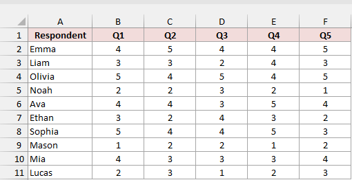
You have the table in A1:F11, with the answers in B2:F11. Each answer is between 1 (strongly disagree) and 5 (strongly agree).

To calculate alpha, you’ll compare how spread out each question’s answers are with how spread out each person’s combined score is. That spread is called variance.

Here is the calculation in plain form:

alpha = k / (k - 1) x (1 - sum of item variances / variance of total scores)

Here, k is the number of questions, also called items. You have five in this survey.

I’ll build this in four small steps:

1. Add each person’s answers to get a total score.

Type Total Score in G1. Enter the following formula in G2 and copy it down to G11:

=SUM(B2:F2)

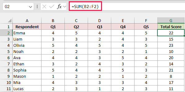
You’ll get these totals, in respondent order: 22, 15, 23, 10, 20, 14, 21, 8, 17, and 11.

SUM adds a row into one value, so you need a separate formula for each respondent.

2. Calculate the variance for each question and the total scores.

I use VAR.S to calculate sample variance, which is the usual choice for survey data.

Type Variance in A12. Enter this formula in B12 and copy it across to G12:

=VAR.S(B2:B11)

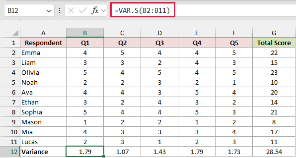
Format B12:G12 to show two decimal places. You’ll see the following variances:

• Q1, in B12: 1.79.
• Q2, in C12: 1.07.
• Q3, in D12: 1.43.
• Q4, in E12: 1.79.
• Q5, in F12: 1.73.
• Total scores, in G12: 28.54.

After copying across, you’ll have =VAR.S(G2:G11) in G12. That’s the total-score variance you’ll use in the final calculation.

3. Count the questions.

Type Number of Items in I1 and Cronbach's Alpha in I2. Leave J2 empty for now, and enter this formula in J1:

=COLUMNS(B1:F1)

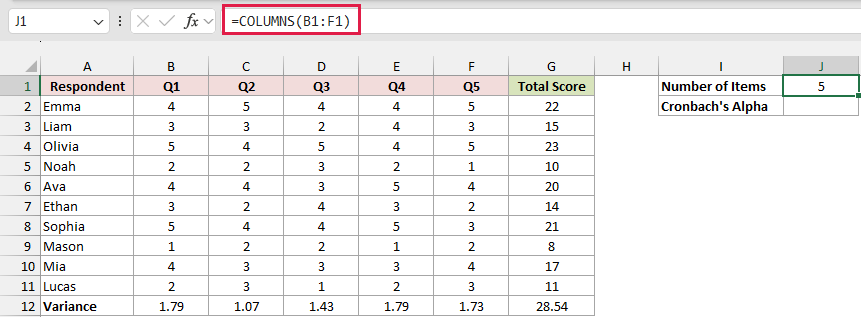
You’ll get 5 because COLUMNS counts the five question columns from B through F. Don’t include the respondent names or Total Score column.

4. Calculate Cronbach’s alpha.

Enter this formula in J2, then format the result to show three decimal places:

=J1/(J1-1)*(1-SUM(B12:F12)/G12)

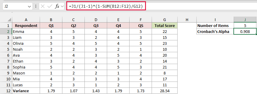
You’ll get 0.908, which indicates a high level of consistency across the five questions.

How does this formula work?

• With SUM(B12:F12), you add the five question variances. Together, they’re about 7.81.
• You divide that by G12, about 28.54, to get approximately 0.274. This is the share of total-score variance from each question varying on its own.
• Subtracting 0.274 from 1 leaves about 0.726.
• With J1/(J1-1), you correct for the number of questions: 5/4 = 1.25. Multiplying 1.25 by about 0.726 returns 0.908.

When people who score high on one question also score high on the others, their total scores spread out more compared with individual questions. Alpha goes up.

Note: You can use VAR.P instead of VAR.S and still get 0.908 if you use it for both the question variances and the total-score variance. The sample adjustment cancels out. Don’t mix VAR.S and VAR.P in one calculation.

Method #2: Using a Single LET Formula

You can also calculate alpha in one cell, without adding a helper column or a variance row.

You’ll need these functions, available in Microsoft 365 and Excel 2024:

• LET to name the parts of your calculation.
• BYCOL to calculate each question’s variance.
• BYROW to add each respondent’s answers.
• LAMBDA to define the small calculation applied to each column or row.

Below I have a dataset of ten customer satisfaction survey responses to five statements, and I want to calculate their consistency in one cell.

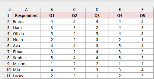
You have the table in A1:F11 and the numeric answers in B2:F11. The ratings run from 1 (strongly disagree) to 5 (strongly agree).

Type Cronbach's Alpha in H1. Enter the following formula in H2 and format the result to show three decimal places:

=LET(data,B2:F11,k,COLUMNS(data),itemVar,SUM(BYCOL(data,LAMBDA(c,VAR.S(c)))),totalVar,VAR.S(BYROW(data,LAMBDA(r,SUM(r)))),k/(k-1)*(1-itemVar/totalVar))

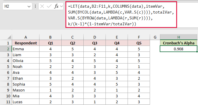
You’ll get 0.908, the same alpha as the step-by-step calculation.

How does this formula work?

I use LET to give names to the answer range and intermediate results:

• data is B2:F11, your block of answers. You leave out respondent names and headers.
• k counts the columns with COLUMNS(data), so you get 5 questions.
• itemVar adds the five question variances, about 7.81. BYCOL applies VAR.S to each column using the small function LAMBDA(c,VAR.S(c)), and SUM adds the results.
• totalVar is about 28.54. BYROW adds each person’s answers using LAMBDA(r,SUM(r)), and VAR.S calculates the variance of those ten totals.
• The final expression, k/(k-1)*(1-itemVar/totalVar), calculates alpha from those named results, just as you did in Method #1.

To reuse the formula for your own survey, change only B2:F11 to your numeric answer range.

Method #3: Using the Analysis ToolPak (ANOVA)

The Analysis ToolPak is a free add-in that comes with desktop Excel for Windows and Mac. You can calculate alpha from its output.

You can use it to compare variation between respondents and questions. This analysis is called ANOVA.

Below I have a dataset of ten customer satisfaction survey responses to five statements, and I want to calculate their consistency using the ToolPak.

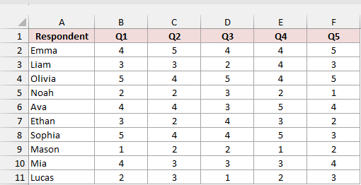
You have the survey table in A1:F11. Each respondent rates five statements from 1 (strongly disagree) to 5 (strongly agree).

Note: If you don’t see Data Analysis on the Data tab, go to File > Options > Add-ins. Choose Excel Add-ins in the Manage box and click Go. Check Analysis ToolPak and click OK. On a Mac, go to Tools > Excel Add-ins, check Analysis ToolPak, and click OK.

Here are the steps to get the values you’ll need for alpha:

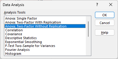
1. Click the Data tab, then click Data Analysis in the Analysis group at the far right.

2. In the Data Analysis dialog, select Anova: Two-Factor Without Replication and click OK.

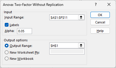
3. In the Anova: Two-Factor Without Replication dialog, enter these settings, then click OK:

• Input Range: $A$1:$F$11, including the respondent names and header row.
• Labels: Check this box.
• Alpha: Leave it at 0.05. This is the ANOVA significance level, not Cronbach’s alpha.
• Output options: Select Output Range and enter $H$1.

You’ll see the output starting in H1. The SUMMARY table lists one row per respondent, followed by one row per question.

Below that, you’ll see an ANOVA table with Rows, Columns, and Error entries.

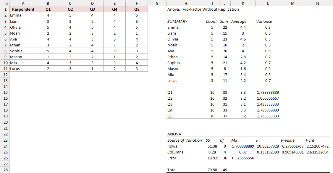
In the ANOVA table, you’ll use the average squared variation, called mean square or MS, for two entries:

• Rows, in K24: 5.709, the spread between respondents.
• Error, in K26: 0.526, the leftover inconsistency.

Type Cronbach's Alpha in P1. Enter the following formula in P2 and format the result to show three decimal places:

=1-K26/K24

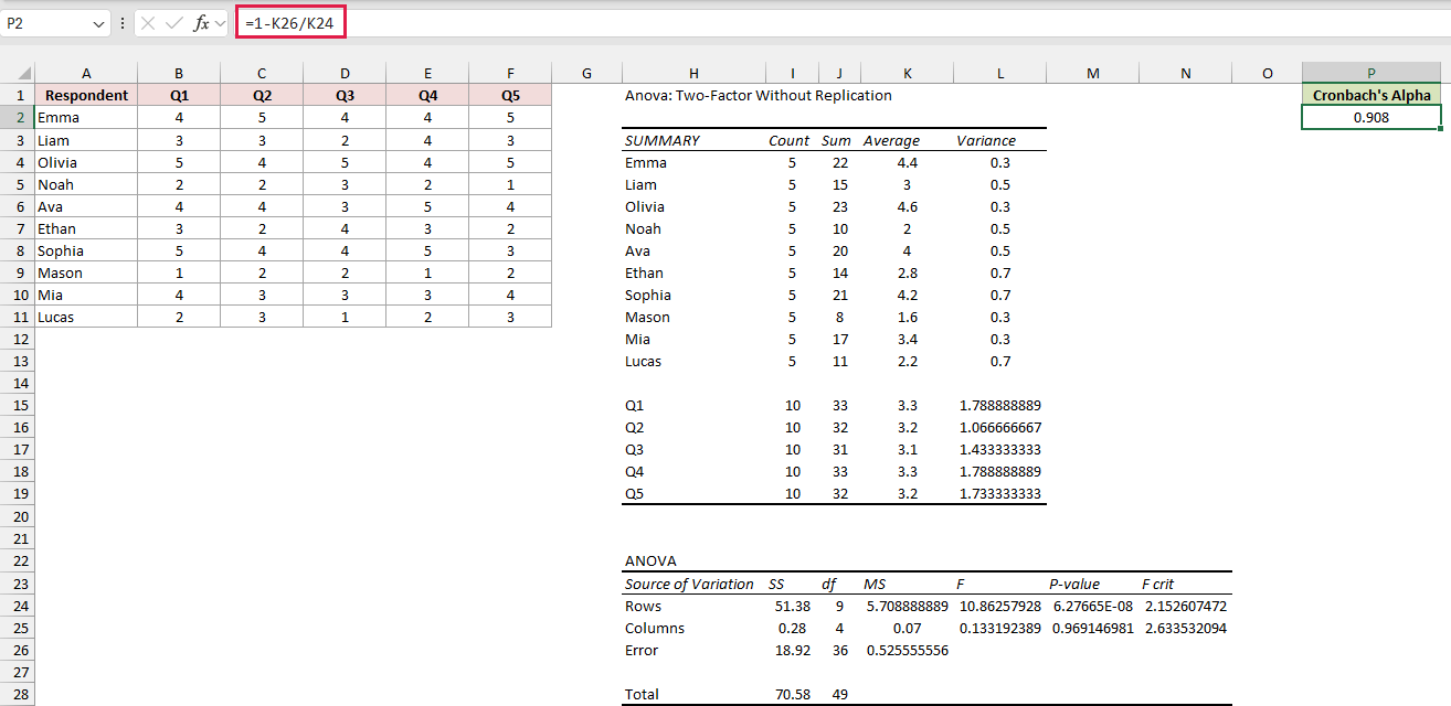
You’ll get 0.908, the same result as both formula methods. Here, you calculate alpha as 1 - MS Error / MS Rows.

Your cell addresses will depend on where you put the output and how many respondents and questions you have. Point at the MS values next to Rows and Error.

The ToolPak returns static numbers, so run it again if your answers change. The formula methods update on their own.

Additional Notes About Calculating Cronbach’s Alpha in Excel

Keep these scoring, layout, and interpretation points in mind when calculating alpha:

• Reverse-score negatively worded questions first. On a 1-to-5 scale, subtract the answer from 6, for example =6-B2. Otherwise, alpha can drop or become negative.
• Keep one row per respondent and one column per question, and use only complete rows. VAR.S skips a blank answer in its column, but SUM still calculates that respondent’s total. Your pieces no longer match.
• Alpha measures how consistently your questions agree. It doesn’t tell you whether they measure the right thing.
• Alpha rises with more questions. A long questionnaire can look reliable even when its questions only loosely agree.

Frequently Asked Questions

Here are a few questions you might have when reporting your survey’s alpha.

What Is a Good Cronbach’s Alpha Value?

You’re checking how consistently the questions agree, often called internal consistency. Use these ranges as a rule of thumb:

Cronbach’s Alpha	Internal Consistency
0.9 and above	Excellent
0.8 to 0.89	Good
0.7 to 0.79	Acceptable
0.6 to 0.69	Questionable
0.5 to 0.59	Poor
Below 0.5	Unacceptable

You can use 0.7 as the common minimum. Our example’s 0.908 falls in the Excellent range.

A value above about 0.95 can mean some questions repeat each other, so a higher alpha isn’t always better.

Does Excel Have a Cronbach’s Alpha Function?

Excel has no built-in function, so use VAR.S and SUM (Method #1) or one LET formula (Method #2).

These formulas recalculate when your answers change, while the ToolPak output stays the same.

How Do I Find Which Question Lowers Alpha?

Recalculate alpha without one question at a time. You’ll often see this called “alpha if item deleted.”

In the Method #2 formula, replace B2:F11 with CHOOSECOLS(B2:F11,1,2,4,5) to leave out Q3.

CHOOSECOLS keeps columns 1, 2, 4, and 5 of your answer range (Q1, Q2, Q4, Q5).

You’ll need Microsoft 365 or Excel 2024 for CHOOSECOLS.

For this survey, you’ll get these results after leaving out each question:

• Without Q1: 0.850.
• Without Q2: 0.881.
• Without Q3: 0.922.
• Without Q4: 0.881.
• Without Q5: 0.896.

Only dropping Q3 raises alpha, from 0.908 to 0.922. That suggests Q3 fits the scale least.

Can Cronbach’s Alpha Be Negative?

Yes. You can get negative alpha when answers to questions move in opposite directions, often because you haven’t reverse-scored a negatively worded question.

Correct the scoring and recalculate alpha.

Conclusion

I recommend Method #1 when you want to see each part of the calculation, in Excel 2010 and later.

Use Method #2 for a one-cell answer in Microsoft 365 or Excel 2024. If you already use the ToolPak, Method #3 lets you calculate alpha from its output.

Other Excel articles you may also like:

• How to Create a Covariance Matrix in Excel