LET Function in Excel

If you want to make a long Excel formula easier to read, the LET function lets you name calculations and reuse them inside that formula.

In Excel 365, LET can work with ranges and spill its final array into the cells below. In this article, I’ll show you six practical ways to use it.

LET Function Syntax in Excel

The LET function pairs each name with a value, then returns the result of a final calculation.

=LET(name1, name_value1, calculation_or_name2, [name_value2, calculation_or_name3...])

• name1 is required. It is the first name you assign and must follow Excel’s rules for defined names.
• name_value1 is required. It is the value or calculation assigned to name1.
• calculation_or_name2 is required. It can be the final calculation or the next name you want to define.
• [name_value2, calculation_or_name3, ...] adds more name and value pairs. The last argument must be a calculation that returns the result.

You can define up to 126 name and value pairs in one LET formula. Each name exists only inside that formula.

When to Use LET Function

• Give meaningful names to cell ranges and intermediate calculations
• Calculate a repeated expression once and reuse its result
• Make nested IF or IFS logic easier to follow
• Break a long dynamic array formula into readable stages
• Return different calculations from the same named inputs

Example 1: Calculate Contract Totals with Named Variables

Let’s start with a formula that names several inputs and one intermediate calculation.

Below is a facility contract list with monthly fees, crew counts, and contract lengths. Column E is where the contract totals will spill.

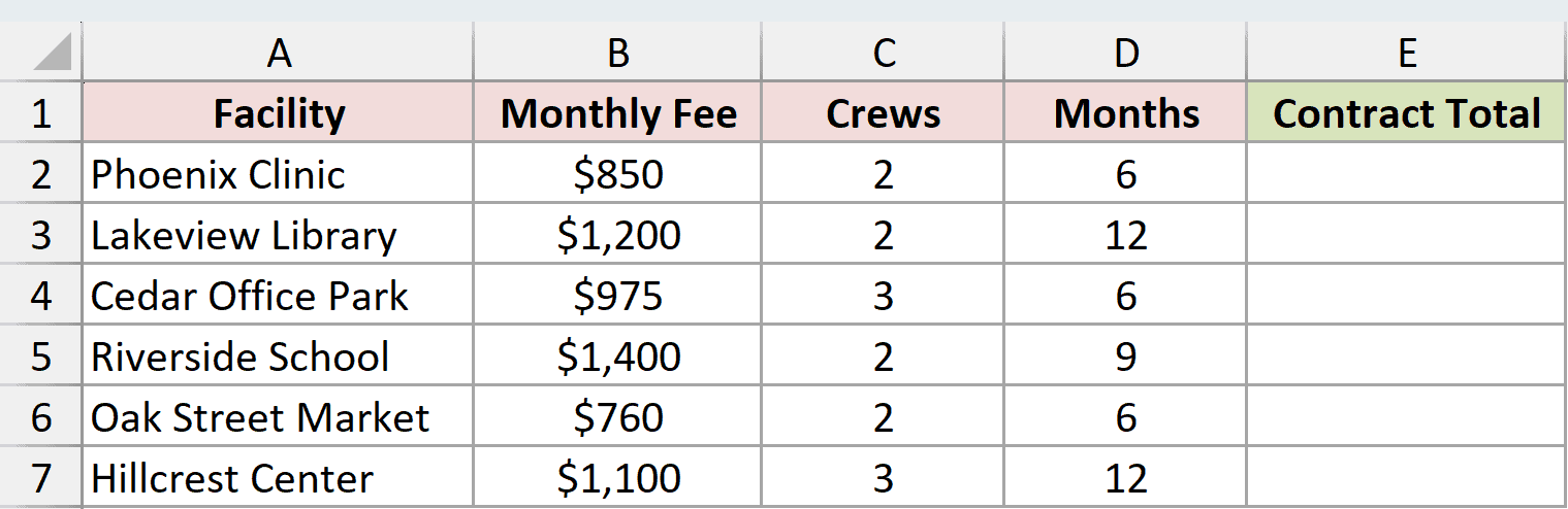
We want to calculate each contract subtotal, apply a 10% discount when that subtotal is at least $15,000, and return the final total.

Here is the formula:

=LET(fee,B2:B7,crews,C2:C7,months,D2:D7,subtotal,fee*crews*months,discount,IF(subtotal>=15000,10%,0),subtotal*(1-discount))

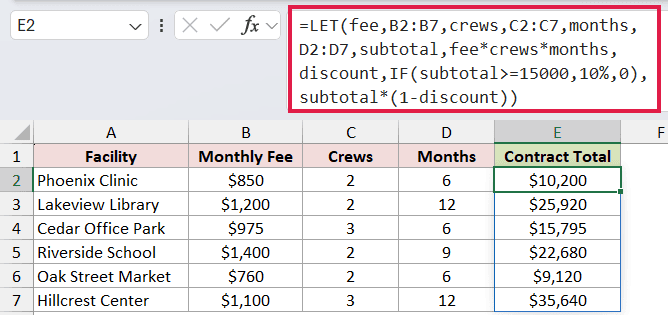
How this formula works:

• fee, crews, and months name the three input ranges.
• subtotal multiplies those named arrays row by row.
• discount returns 10% for subtotals of $15,000 or more, and 0 for the rest.
• The final calculation applies the discount and spills six totals into E2:E7.

Phoenix Clinic stays at $10,200 because it does not reach the threshold. Lakeview Library receives the discount and returns $25,920.

Example 2: Reuse a Delay Calculation

Here’s a short example where LET saves us from repeating the same subtraction.

Below is a service-job table with target minutes in column B and actual minutes in column C. Column D will show the SLA result.

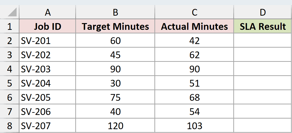
We want to label late jobs with the number of minutes delayed and show “On time” for everything else.

Here is the formula:

=LET(delay,C2:C8-B2:B8,IF(delay>0,delay&" min late","On time"))

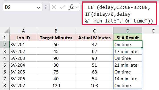
The name delay stores the difference between actual and target minutes for all seven jobs. The IF function then tests that array and uses the same name again when it builds the late labels.

SV-202 returns “17 min late,” while SV-203 returns “On time” because its actual time matches the target.

Pro Tip: A LET name does not become a workbook-level defined name. It exists only while Excel evaluates that LET formula.

Example 3: Name an XLOOKUP Result

Now let’s reuse the result of a lookup instead of running the same lookup more than once.

Below is a van service table. Each route type has a service interval in F2:G4, and column D will show how far each van is from its next service.

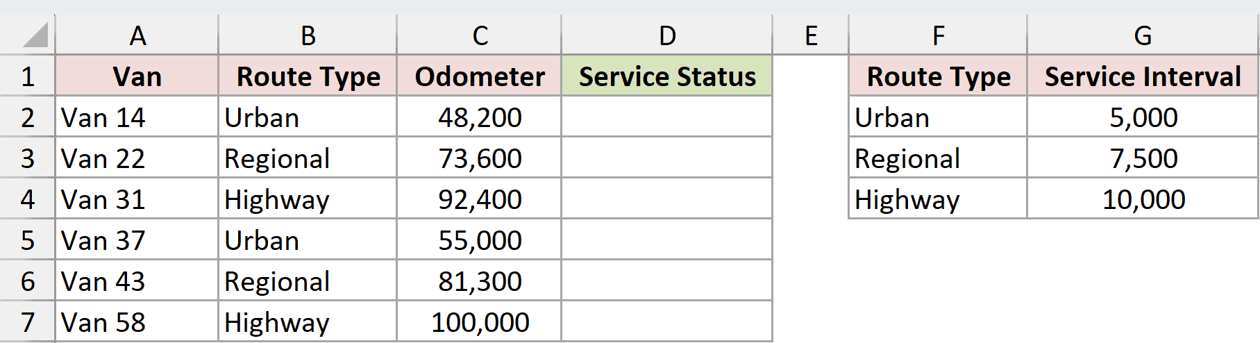
We want to find each route’s interval once, use it to calculate the remaining miles, and return a clear service status.

Here is the formula:

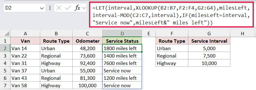
=LET(interval,XLOOKUP(B2:B7,F2:F4,G2:G4),milesLeft,interval-MOD(C2:C7,interval),IF(milesLeft=interval,"Service now",milesLeft&" miles left"))

How this formula works:

• interval stores the service interval returned by XLOOKUP for each route type.
• milesLeft uses the MOD function to subtract the odometer remainder from that interval.
• The final IF shows “Service now” when the odometer lands exactly on an interval. Otherwise, it shows the remaining miles.

Van 14 returns “1800 miles left.” Van 37 and Van 58 both return “Service now.”

Example 4: Filter and Sort Supply Shortfalls

LET is especially handy when one dynamic array step feeds another.

Below is a supply request table with on-hand and needed quantities. The three-column result will spill from G2.

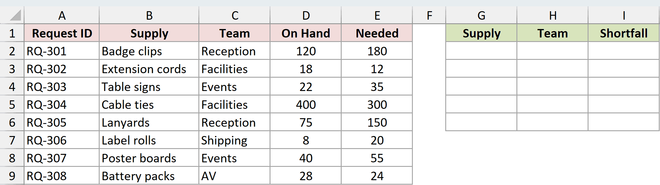
We want a report containing only shortages, sorted from the largest shortfall to the smallest.

Here is the formula:

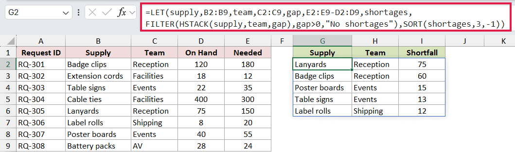
=LET(supply,B2:B9,team,C2:C9,gap,E2:E9-D2:D9,shortages,FILTER(HSTACK(supply,team,gap),gap>0,"No shortages"),SORT(shortages,3,-1))

How this formula works:

• gap calculates needed minus on-hand quantities.
• HSTACK combines the supply, team, and gap arrays into three columns.
• FILTER keeps only rows where gap is greater than zero and stores them as shortages.
• SORT uses column 3 in descending order, so the biggest shortage appears first.

The result begins with Lanyards at 75 and ends with Label rolls at 12. Because the result spills, the cells in G2:I6 must be empty before you enter the formula.

This example needs Excel 365 or Excel 2024 because HSTACK is not available in Excel 2021.

Example 5: Simplify a Multi-Condition Action Rule

Here’s a case where names make a longer set of business rules much easier to inspect.

Below is a permit list with fees, days remaining, and risk levels. Column F will show the action for each permit.

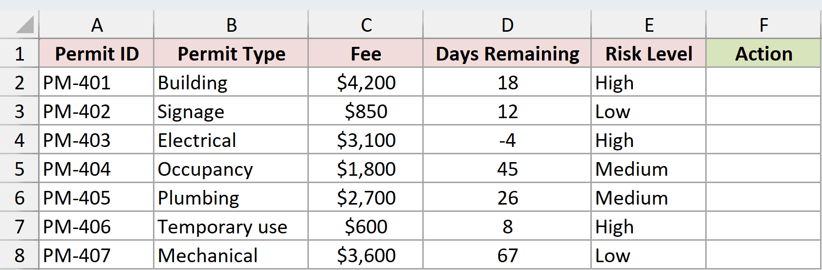
We want to flag expired permits first, then prioritize high-fee or high-risk permits that expire within 30 days.

Here is the formula:

=LET(fee,C2:C8,daysLeft,D2:D8,risk,E2:E8,priority,(fee>=2500)+(risk="High"),IFS(daysLeft<0,"Expired",(daysLeft<=30)*(priority>0),"Call now",daysLeft<=30,"Email reminder",TRUE,"No action"))

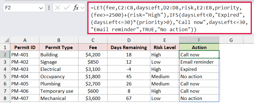
The first three names point to the input columns. priority becomes positive when the fee is at least $2,500, the risk is High, or both conditions are true.

The IFS function checks the rules in order. That order matters because an expired permit must return “Expired” before Excel considers any reminder action.

PM-403 is expired. PM-401, PM-405, and PM-406 return “Call now,” while PM-402 gets an email reminder.

Example 6: Reuse Revenue and Profit Calculations

For the last example, we’ll use the same named calculation in two related results.

Below is a workshop table with registrations, attendance rates, fees, and venue costs. Columns F and G will show the margin and a revenue check.

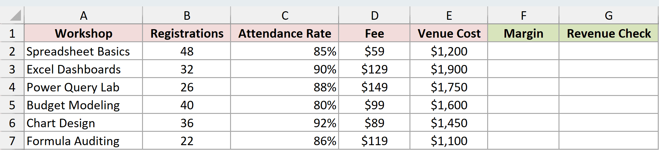
We first want each workshop’s profit margin, with revenue and profit calculated only once inside the formula.

Here is the margin formula:

=LET(revenue,B2:B7*C2:C7*D2:D7,profit,revenue-E2:E7,IFERROR(profit/revenue,0))

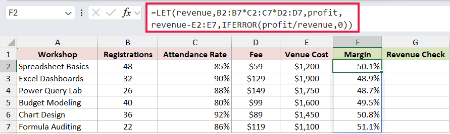
revenue multiplies registrations, attendance rate, and fee. profit subtracts venue cost, and the final calculation divides profit by revenue. IFERROR returns 0 if revenue is zero.

The first workshop returns a 50.1% margin after Excel applies the percentage format in column F.

We can also return the named revenue calculation itself to check the figures.

Here is the revenue-check formula:

=LET(revenue,B2:B7*C2:C7*D2:D7,profit,revenue-E2:E7,revenue)

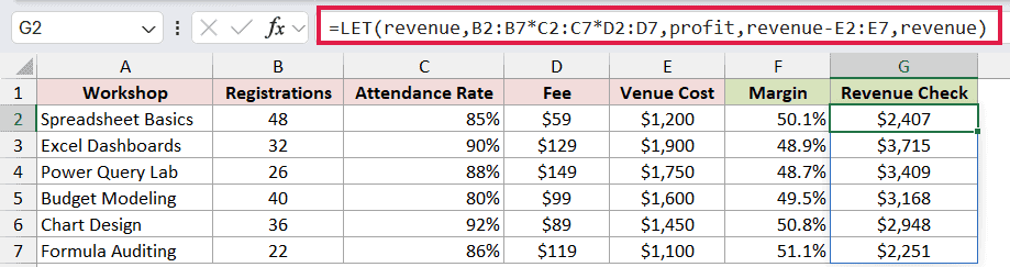
The two formulas define the same names, but their final arguments differ. The first returns IFERROR(profit/revenue,0), while the second returns revenue.

For Spreadsheet Basics, the revenue check is $2,407.20. LET returns only its last calculation, even when it defines several names beforehand.

Pro Tip: Choose short, descriptive names such as revenue, profit, or daysLeft. A name like c is invalid because it conflicts with Excel’s R1C1 reference style.

Tips & Common Mistakes

• The last LET argument must be a calculation that returns a result. Do not end the formula with a name that still needs a value.
• LET names follow Excel’s defined-name rules. They must start with a letter and cannot look like a cell reference.
• A name is available only after you define it. A later name can use an earlier one, but not the other way around.
• LET is available in Excel 2021, Excel 2024, and Microsoft 365. It is not available in Excel 2019 or earlier.
• A spilled LET result needs a clear output range. If another value blocks it, Excel returns #SPILL!.
• LET improves readability and can avoid recalculating a repeated expression. It does not automatically make every short formula better.

LET is useful when a formula repeats work or becomes hard to read. I hope you found these examples helpful and can use the same naming pattern in your own formulas.

List of All Excel Functions

Related Excel Functions / Articles:

• LAMBDA Function in Excel
• MAP Function in Excel
• IF Function in Excel
• SWITCH Function in Excel
• CHOOSE Function in Excel