
When a regular filter checklist isn’t specific enough, Custom AutoFilter lets you filter a column with operators such as Contains, Begins With, Between, and After.
That helps when you’re looking for products containing Desk, amounts between two limits, or orders after a cutoff date. You can join two tests with And or Or.
I’ll show you text and wildcard filters, And and Or number filters, and date filters.
You’ll also learn how to handle three or more conditions with Advanced Filter or FILTER.
How to Open the Custom AutoFilter Dialog Box
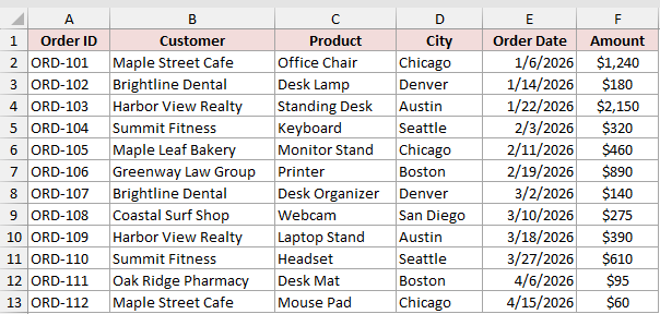
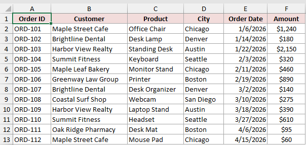
I’ll use the Orders sheet, where the dataset occupies A1:F13. It contains 12 orders with customer, product, city, date, and amount details.
Here are the steps to open the Custom AutoFilter dialog box:
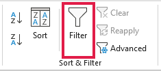
- Select A1:F13. On the Data tab, click Filter. You can also press Ctrl+Shift+L, or Cmd+Shift+F on a Mac.
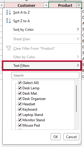
- Open a column’s filter arrow. Point to Text Filters, Number Filters, or Date Filters, then select Custom Filter.
The dialog has two condition rows. Select And when both conditions must be true, or Or when either condition may be true.
Method #1: Using Text Filters (Contains and Begins With)
Text Filters are the quickest choice when you need a partial text match. Use Contains for text anywhere in a cell and Begins With for text at the start.
On the Orders sheet, I want to find products whose names contain or begin with the word Desk.
Here are the steps to apply the two text filters:
- Open the Product filter arrow, point to Text Filters, and select Contains.
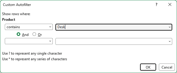
- Enter
Deskand click OK.
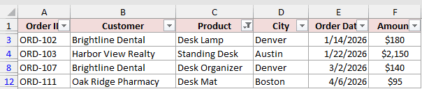
Excel shows ORD-102, ORD-103, ORD-107, and ORD-111. Their products are Desk Lamp, Standing Desk, Desk Organizer, and Desk Mat.
- Reopen the Product filter. Choose Text Filters, Begins With, enter
Desk, and click OK.

The second filter returns ORD-102, ORD-107, and ORD-111. Standing Desk drops out because its product name doesn’t begin with Desk.
Method #2: Using Wildcards (* and ?)
Wildcards let one criterion stand in for unknown characters, so they’re useful when several values follow the same text pattern.
On the Orders sheet, I’ll first find product names containing Stand. Then I’ll match order IDs with one unknown final character.
Here are the steps to use both wildcard characters:
- Open the Product filter. Choose Text Filters, Custom Filter, set the operator to equals, enter
*Stand*, and click OK.

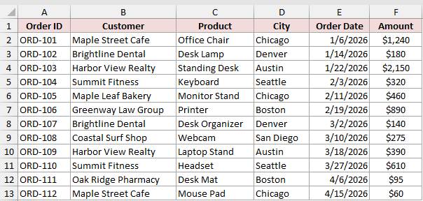
The asterisks allow any number of characters before and after Stand. Excel returns ORD-103, ORD-105, and ORD-109.
- Clear that filter. Open the Order ID filter arrow, point to Text Filters, and select Custom Filter. Set equals to
ORD-10?, then click OK.
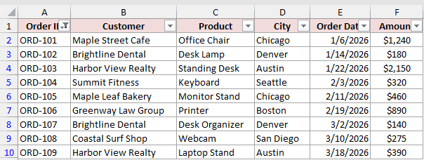
The question mark represents exactly one character. The filter returns ORD-101 through ORD-109 and hides ORD-110 through ORD-112.
Note: To search for a literal asterisk or question mark, place a tilde before it. Use ~* for an asterisk or ~? for a question mark.
Method #3: Using the And Option
If a number must satisfy a lower and upper limit, join the conditions with And. Both tests must be true for a row to remain visible.
On the Orders sheet, I want amounts from $300 through $1,000, including both limits.
Here are the steps to filter the Amount column:
- Clear the Order ID filter. Open the Amount filter arrow. Point to Number Filters and select Between.
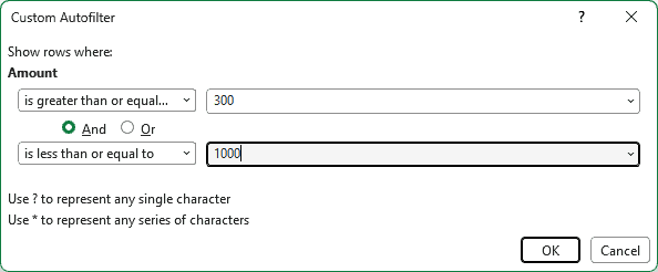
- Set the first condition to is greater than or equal to
300. Select And, set the second to is less than or equal to1000, and click OK.
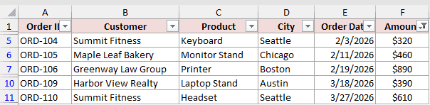
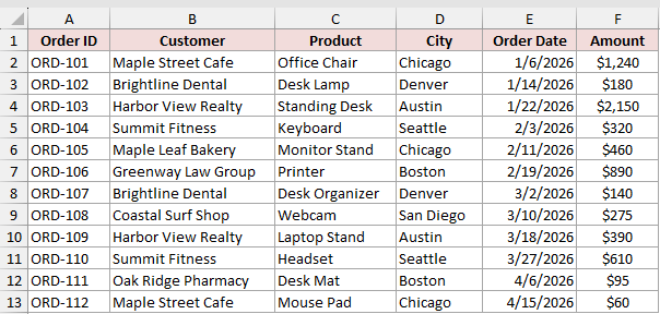
Excel returns ORD-104, ORD-105, ORD-106, ORD-109, and ORD-110. Every visible amount is at least $300 and no more than $1,000.
Method #4: Using the Or Option
Use Or when a row may satisfy either test. This works well for two cities, two labels, or two separate numeric bands in one column.
On the Orders sheet, I’ll first keep orders from Chicago or Denver. Then I’ll show a second example using the Amount column.
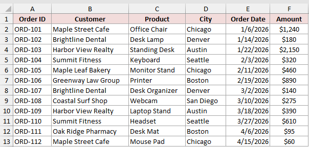
Here are the steps to apply the two OR filters:
- Clear the Amount filter. Open the City filter and choose Text Filters, Custom Filter. Set equals to
Chicago, select Or, set the second equals toDenver, and click OK.
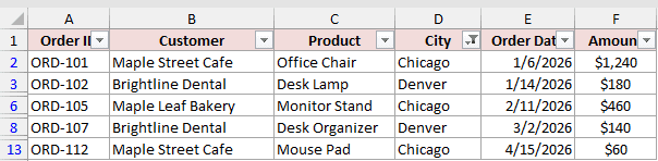
Excel returns ORD-101, ORD-102, ORD-105, ORD-107, and ORD-112 because each order belongs to one of those cities.
- Clear the City filter. Open the Amount filter arrow, point to Number Filters, and select Custom Filter. Set the first condition to is greater than or equal to
1000, select Or, set the second to is less than100, and click OK.
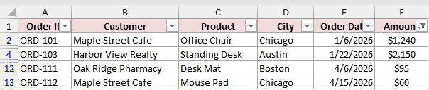
The second filter returns ORD-101, ORD-103, ORD-111, and ORD-112. An amount needs to meet only one side of the OR test.
Method #5: Using Custom AutoFilter on Dates
Date Filters use the same two-condition dialog with date-specific operators. Use this route when you need an inclusive range or a cutoff date.
On the Orders sheet, I want orders dated from February 1 through March 31, 2026.
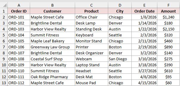
Here are the steps to create the date filters:
- Clear the Amount filter. Open the Order Date filter. Choose Date Filters, Between. Set is after or equal to
2/1/2026And is before or equal to3/31/2026, then click OK.
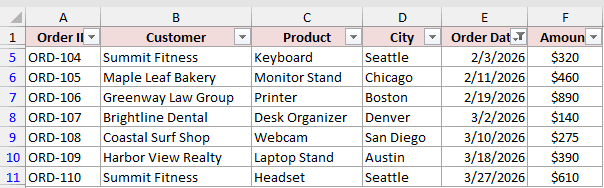
Excel returns ORD-104 through ORD-110, which gives seven orders inside the inclusive date range.
- Clear that filter. Choose Date Filters, After, enter
3/1/2026, and click OK.
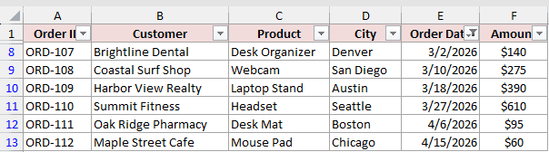
The second filter returns ORD-107 through ORD-112 because each order is dated after March 1, 2026. The earliest is ORD-107 on March 2.
Note: Type dates in the format your system uses. On a day/month system, February 1, 2026 is 1/2/2026 rather than 2/1/2026.
Method #6: Using Advanced Filter (More Than Two Conditions)
Custom AutoFilter allows only two conditions per column. Advanced Filter is the built-in alternative when you need three or more conditions on one column.
On the Advanced Filter sheet, the list is in A1:F13. H1:H4 contains Product, *Desk*, *Stand*, and *Chair*.
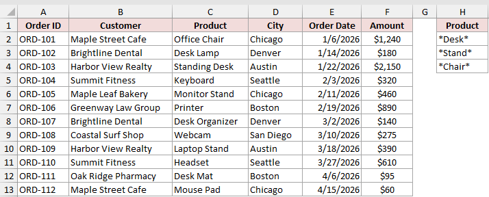
Here are the steps to filter the list in place:
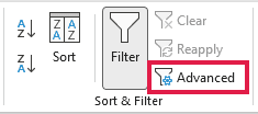
- Select a cell in A1:F13. On the Data tab, click Advanced in the Sort & Filter group.
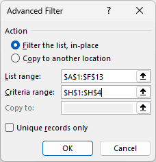
- Select Filter the list, in-place. Set List range to
$A$1:$F$13and Criteria range to$H$1:$H$4.
- Click OK.
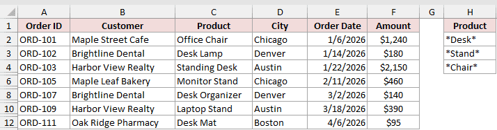
Excel keeps ORD-101, ORD-102, ORD-103, ORD-105, ORD-107, ORD-109, and ORD-111 visible.
Each criterion occupies a separate row under the same Product heading. In an Advanced Filter criteria range, separate rows work as OR conditions.
Method #7: Using the FILTER Function
When you need a live result with more than two conditions, the FILTER function can return matching rows elsewhere and update when the source changes.
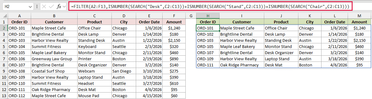
Below I have the 12-order dataset on the FILTER Function sheet. I want to return products containing Desk, Stand, or Chair.
The source data is in A1:F13. The result starts in H2 and spills through M8.
Enter this formula in H2:
=FILTER(A2:F13,ISNUMBER(SEARCH("Desk",C2:C13))+ISNUMBER(SEARCH("Stand",C2:C13))+ISNUMBER(SEARCH("Chair",C2:C13)))
How does this formula work?
The three SEARCH functions look for Desk, Stand, or Chair in each product name. ISNUMBER converts each successful search into TRUE.
Adding those arrays makes the plus signs act like OR. FILTER keeps a row whenever at least one search produces a number.
The formula spills the same seven orders into H2:M8: ORD-101, ORD-102, ORD-103, ORD-105, ORD-107, ORD-109, and ORD-111.
Note: The FILTER function is available in Microsoft 365 and Excel 2021 or later. Use Advanced Filter when your Excel version doesn’t support it.
Additional Notes About Using Custom AutoFilter in Excel
- The Text Filters, Number Filters, or Date Filters menu depends on the column’s data type. Numbers stored as text display Text Filters.
- Custom AutoFilter accepts two conditions per column. Filters applied to several columns combine as AND, so every column’s filter must pass.
- Wildcards work with text. Use
~*or~?when you need to find the actual symbol. - Text criteria are not case-sensitive.
desk,Desk, andDESKmatch the same text. - Use Data > Clear to clear criteria while keeping the arrows. Ctrl+Shift+L removes the filtering buttons.
Frequently Asked Questions
How Do I Use More Than Two Conditions in Custom AutoFilter in Excel?
The Custom AutoFilter dialog stops at two conditions per column. Use Advanced Filter for criteria on separate rows, or FILTER for a live result in newer Excel versions.
What Is the Difference Between AND and OR in Custom AutoFilter?
And keeps a row only when both conditions are true. Or keeps a row when either condition is true.
How Do I Filter With Wildcards in Excel?
Use * for any number of characters and ? for exactly one character. Prefix either symbol with ~ when you need a literal match.
How Do I Clear a Custom Filter in Excel?
Click Data > Clear to remove the criteria but keep the filter arrows. Press Ctrl+Shift+L if you’d also like to remove the arrows.
Why Is My Custom AutoFilter Not Showing All Results?
If you’re still missing rows, check for numbers stored as text, mixed data types, blank rows, merged cells, and an incomplete filter range.
Also confirm that your And or Or choice matches the intended logic.
Conclusion
In this article, I showed you how to use Custom AutoFilter with text, wildcard, number, and date conditions, joined with And or Or.
I also covered Advanced Filter and the FILTER function for more than two conditions. I hope you found this article helpful.
Other Excel articles you may also like:
