
Need just one month’s records from your Excel log, or everything between two dates? I’ll show you how to filter that date column without removing the other records.
For quick filters, we’ll use the header arrows. For a separate result that updates when you change your dates, I’ll walk you through the formulas.
For older versions, I’ll also show you how to copy matching rows with Excel’s Advanced Filter.
Method #1: Using the Date List in the Filter Drop-Down
For a whole month’s records, pick a year and month from the date column’s drop-down. That saves you typing a start or end date.
Below I have a dataset of equipment rentals in A1:D15 on the Rentals sheet, and I want to see only March 2026.
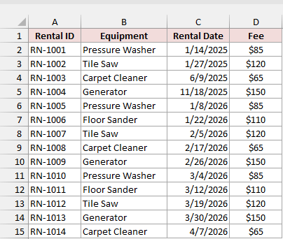
I’ll turn on the header arrows first, then choose the month I need.
- Select any cell in the data. On the Data tab, click Filter in the Sort & Filter group.
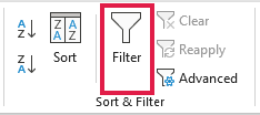
Each header now has an arrow. For a shortcut, you can turn these arrows on with Ctrl + Shift + L.
- Click the arrow in the Rental Date header.
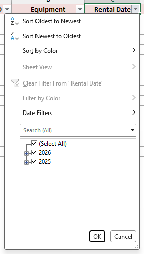
Here, you’ll find separate groups for 2026 and 2025. Expand a year to see its months, then a month to see individual days.
- Uncheck (Select All). Click the small plus sign next to 2026, then check March.
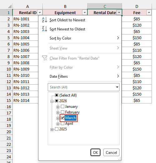
- Click OK.
With March 2026 selected, you’re left with four rentals, RN-1010 through RN-1013.
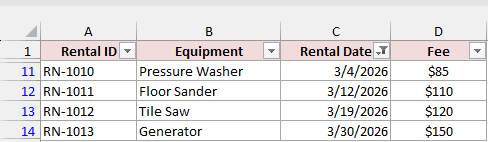
The other rentals are still there, just hidden. Look for the blue row numbers and funnel icon to tell you the filter is active.
Need more than one period? Check several months or years in the same drop-down.
Note: If your real dates appear individually, turn on Group dates in the AutoFilter menu under File > Options > Advanced > Display options for this workbook.
Method #2: Using the Between Date Filter
When you need a date range rather than a whole month, I recommend the built-in Between filter for most people.
There’s no formula to write, and your results include records on both the start and end dates.
Below I have a dataset of equipment rentals in A1:D15 on the Rentals sheet, and I want rentals from 2/10/2026 through 3/15/2026.
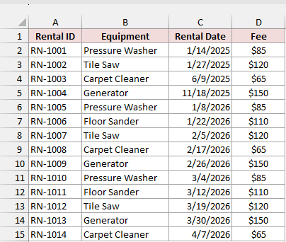
Before you start, make sure the filter arrows are on. You can press Ctrl + Shift + L if they’re missing.
I’ll enter the two dates using these steps.
- Click the Rental Date arrow, point to Date Filters, then click Between….
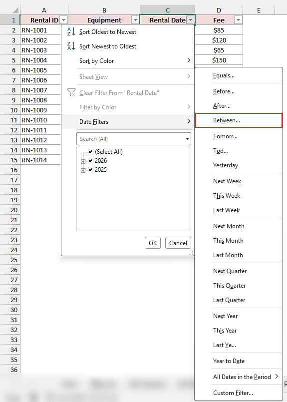
The same submenu also gives you ready-made periods:
- Today
- This Week
- Last Month
- This Quarter
- Year to Date
After choosing Between, you’ll enter both date conditions in the Custom AutoFilter dialog box.
- Enter 2/10/2026 beside is after or equal to. Keep And selected, then enter 3/15/2026 beside is before or equal to. You can also use the calendar buttons.
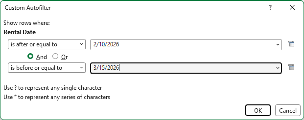
Leave And selected rather than Or so your results meet both conditions.
- Click OK.
For this range, you’ll see four rentals dated from 2/17/2026 to 3/12/2026.
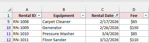
Your results include RN-1008 dated 2/17/2026, RN-1009 dated 2/26/2026, RN-1010 dated 3/4/2026, and RN-1011 dated 3/12/2026.
Because both conditions include equality, you’d also keep rentals dated exactly 2/10/2026 or 3/15/2026.
Note: Ready-made periods such as Today and Last Month use today’s date. You can make Excel check them again by choosing Data > Reapply.
Method #3: Using All Dates in the Period (Any Year)
Sometimes I want every January rental across the years in my log. This option lets you choose a month without choosing a year.
Below I have a dataset of equipment rentals in A1:D15 on the Rentals sheet, including January dates in both 2025 and 2026.
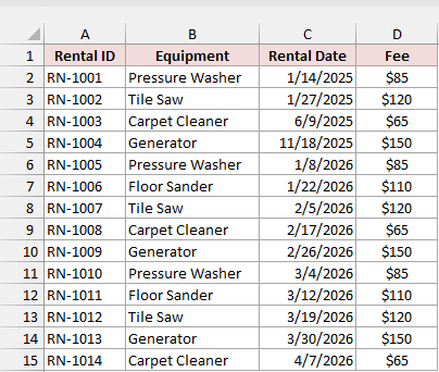
Before you start, make sure the filter arrows are on. You can press Ctrl + Shift + L if they’re missing.
Here’s how I select January from both years.
- Click the Rental Date arrow. Point to Date Filters, then All Dates in the Period, and click January.
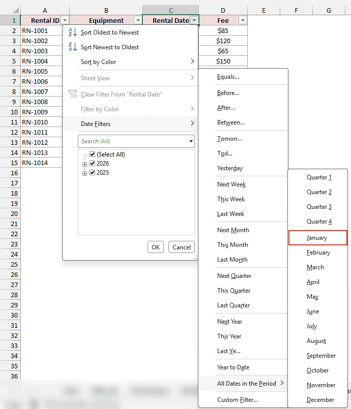
That leaves you with four January rentals, two from 2025 and two from 2026.
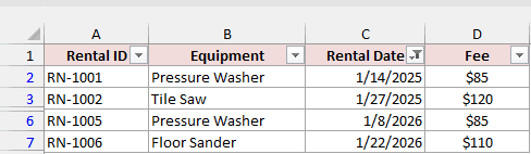
Your January results include RN-1001 dated 1/14/2025, RN-1002 dated 1/27/2025, RN-1005 dated 1/8/2026, and RN-1006 dated 1/22/2026.
Any month in this submenu works the same way. If you choose Quarter 1 through Quarter 4, those choices ignore the year too.
Method #4: Using the FILTER Function for a Date Range
If you want matching rentals in a separate area, a formula can pull them there while keeping your original rows visible.
For this method, you’ll need the FILTER function in Microsoft 365 or Excel 2021 and later.
I want rentals from 1/1/2026 through 2/28/2026.
Below I have a dataset of equipment rentals on the FILTER Date Range sheet, with Start Date and End Date inputs above the table.
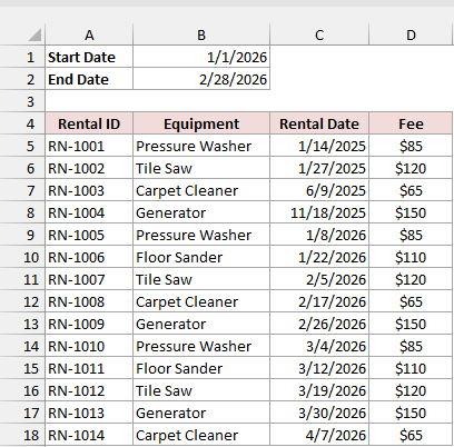
My source headers are in A4:D4 and rental records in A5:D18. I’ve put the same four headers in F4:I4 for your result.
Enter 1/1/2026 in B1 and 2/28/2026 in B2, then put this formula in F5.
=FILTER(A5:D18,(C5:C18>=B1)*(C5:C18<=B2),"No rentals found")
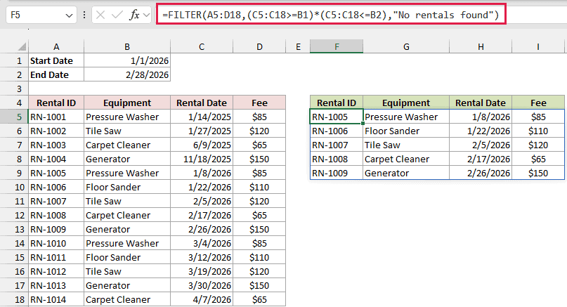
How does this formula work?
The first part, A5:D18, tells FILTER which rental records I want to return, including all four columns.
For your start date, C5:C18>=B1 checks each rental date and returns TRUE for dates on or after 1/1/2026.
At the other end, C5:C18<=B2 returns TRUE for dates on or before 2/28/2026.
Multiplying the tests makes them act like AND. Only rows where both are TRUE give you 1 and pass the check.
I’ve included "No rentals found" as the message when nothing matches. Change your start date to 1/1/2027 and you’ll see it.
With these inputs, you’ll get five rentals, RN-1005 through RN-1009, covering January and February 2026.
Enter the formula only in F5. Your matching rows fill the cells below automatically, a behavior called spilling, so there’s no need to drag the formula down.
Changing B1 or B2 updates your result automatically. Both end dates are included because I’ve used >= and <= in the formula.
Note: FILTER doesn’t copy the source date format. If you see a number such as 46030 for 1/8/2026, format column H as a date. I already have that formatting in the sample file.
Method #5: Using FILTER With MONTH and YEAR
For a separate result covering one month in a specific year, I combine FILTER with MONTH and YEAR.
MONTH gives me each date’s month number, and YEAR gives me its four-digit year. You can use both checks inside FILTER in Microsoft 365 or Excel 2021 and later.
Here, I want March 2026 rentals, so my inputs are month number 3 and year 2026.
Below I have a dataset of equipment rentals on the FILTER Month sheet, with Month and Year inputs above the table.
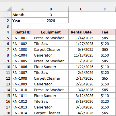
My source headers are in A4:D4 and records in A5:D18. I’ve put the same headers in F4:I4 for your separate result.
Enter 3 in B1 and 2026 in B2, then put this formula in F5.
=FILTER(A5:D18,(MONTH(C5:C18)=B1)*(YEAR(C5:C18)=B2),"No rentals found")
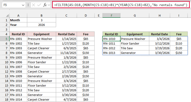
How does this formula work?
First, MONTH(C5:C18) returns each rental date’s month number, from 1 to 12. Comparing those numbers with B1 gives you March, month 3.
Next, YEAR(C5:C18) returns each date’s four-digit year. I compare those years with B2 to keep 2026.
Multiplying the checks means both must be TRUE. Your results include March 2026 rentals rather than every March rental regardless of year.
FILTER returns your matching rows from A5:D18. I’ve included "No rentals found" for cases where no rental matches both inputs.
With these inputs, you’ll see four March 2026 rentals, RN-1010 through RN-1013, spilling from F5 automatically.
For January in another year, change B1 to 1 and B2 to 2025. You’ll get RN-1001 and RN-1002 without editing the formula.
If column H shows numbers instead of dates, apply the date formatting I’ve already set in the sample file.
Method #6: Using Advanced Filter
Even in an older Excel version, you can copy matching rentals to another area without a formula.
With Advanced Filter, you write date conditions in worksheet cells, then ask Excel to apply them. This method works in every Excel version.
I want rentals from 11/1/2025 through 1/31/2026.
Below I have a dataset of equipment rentals in A1:D15 on the Advanced Filter sheet, with the date conditions in F1:G2.
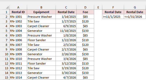
Your conditions sit in a few cells on the sheet. Here, I’ve used F1:G2, which Excel calls the criteria range.
In both F1 and G1, type Rental Date exactly as it appears in your source header.
For this example, I enter >=11/1/2025 in F2 and <=1/31/2026 in G2. When you type the dates, use your computer’s date format.
Keep the conditions side by side on the same row so each rental must pass both.
Repeating the Rental Date header lets you apply both conditions to that column.
I’ll copy the matching rows using these steps.
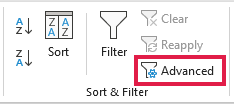
- Select any cell in the data. On the Data tab, click Advanced in the Sort & Filter group.
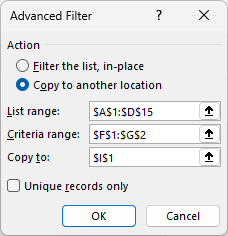
- In the Advanced Filter dialog box, select Copy to another location. Set List range to $A$1:$D$15, Criteria range to $F$1:$G$2, and Copy to to $I$1.
- Click OK.
Excel copies your three matching rentals into I1:L4, including the column headers in I1:L1.
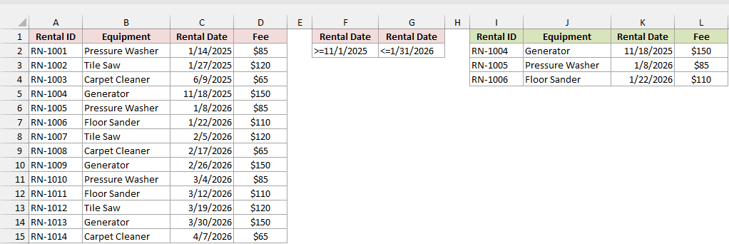
Below your copied headers, you’ll find these rental records:
- RN-1004, Generator, dated 11/18/2025, with a $150 fee.
- RN-1005, Pressure Washer, dated 1/8/2026, with an $85 fee.
- RN-1006, Floor Sander, dated 1/22/2026, with a $110 fee.
To hide the non-matching rows in your original list, choose Filter the list, in-place instead.
Note: You get a fixed copy of the matching rows. Run Advanced Filter again after you change the source data or the criteria.
Additional Notes About Filtering by Date in Excel
Before you filter, I recommend checking a few details that can cause problems.
- Dates stored as text usually sit on the left. Select the column, choose Data > Text to Columns, and click Finish to convert them.
- A blank row can stop Excel from including the rest of your log. Remove blank rows or select the whole range before turning on Filter.
- To show everything again, use Data > Clear. To clear only the date filter, open its arrow and choose Clear Filter From “Rental Date”.
- Filtering hides the rows you don’t want to see. It doesn’t delete them, so you can bring them back by clearing the filter.
Frequently Asked Questions
I’ll answer a few questions you may run into when filtering dates.
Why is my date filter not grouping by month?
You may have dates stored as text. If you see Text Filters instead of Date Filters, convert the column using Data > Text to Columns.
From there, click Next twice, choose Date and MDY for month/day/year text, then click Finish.
For a quick check, try ISNUMBER on a date cell. A real date gives you TRUE.
If you have real dates, enable Group dates in the AutoFilter menu under File > Options > Advanced > Display options for this workbook.
How do I filter dates for this month or last month?
Open your date column’s arrow, point to Date Filters, and choose This Month or Last Month.
These options use today’s date as the reference point. When you want Excel to check the period again, choose Data > Reapply.
How do I filter a date range in a PivotTable?
Add a date slicer called a Timeline using Insert > Timeline. With it, you can filter by months or quarters, or select years.
Does the FILTER function include both the start and end date?
Yes, you include both dates when your formula uses >= for the start and <= for the end.
To exclude the two end dates, use > and < instead.
Conclusion
I’d use the Between filter for a quick date range because you can set both dates without writing a formula.
I’d choose FILTER when you want a separate result that updates as you change the date inputs.
Other Excel articles you may also like:
