
If you want to find the order size that minimizes relevant annual ordering and holding costs, the EOQ formula is what you need. EOQ stands for Economic Order Quantity, and it balances those two costs.
Order in small batches and you place more orders, so ordering costs climb. Order in huge batches and you sit on stock, so holding costs climb. The EOQ is the sweet spot between the two.
Excel has no EOQ button, but the formula is a one-line SQRT you can set up in a minute.
I’ll show you three ways to calculate EOQ in Excel: a direct formula for one item, a spilling formula for your whole inventory, and a Data Table that confirms the result.
Method #1: Using the EOQ Formula
The fastest way is to type the EOQ formula straight into a cell using your three inputs. This works for any single item you’re planning to reorder, so it’s the one I reach for most.
Say I run a home-building supply store and I’m planning orders for interior doors.
For this example, D is 2,000 doors per year, S is $75 per order, and H is $30 per door per year. The EOQ result is doors per order. Here are those inputs in a sheet:
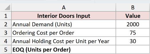
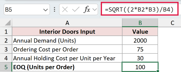
With demand in B2, ordering cost in B3, and holding cost in B4, here is the formula:
=SQRT((2*B2*B3)/B4)
How does this formula work?
The EOQ formula multiplies the annual demand by the ordering cost, doubles it, and divides that by the holding cost. So 2*B2*B3 gives me 300,000, and dividing by the holding cost of 30 gives 10,000.
SQRT then takes the square root of 10,000, which is 100. The EOQ is 100 doors per order. Under the basic model, that quantity minimizes the total relevant annual ordering and holding cost.
Method #2: Applying a Spilling Formula
The formula above handles one product at a time. Most stores track their whole inventory in one table, and copying a formula into every row by hand gets old fast. A single spilling formula can calculate the EOQ for every item at once.
Here’s my inventory list in a normal worksheet range. Each row is a different product, with its annual demand, ordering cost, and holding cost. I want an EOQ for each one in column E.
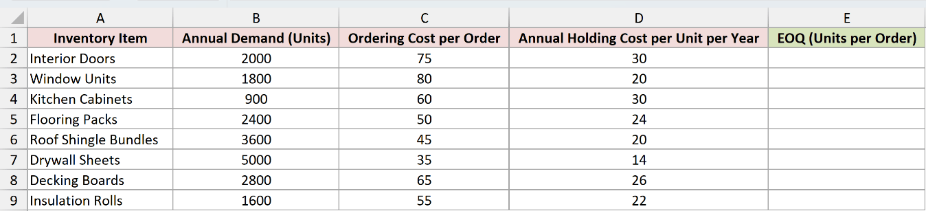
I type the formula once in cell E2 and point each part at the whole column instead of a single cell:
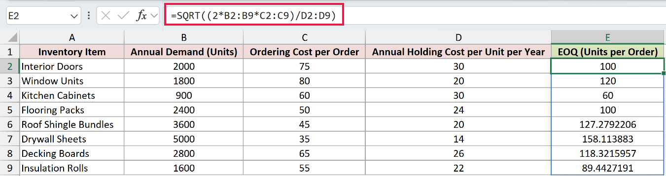
=SQRT((2*B2:B9*C2:C9)/D2:D9)
How does this formula work?
Because I fed it ranges instead of single cells, Excel runs the same math on every row. It multiplies each row’s demand and ordering cost by 2, divides by that row’s holding cost, and takes the square root.
The formula spills down the column automatically, so one entry in E2 fills the EOQ for all eight products. Interior doors come out at 100, window units at 120, kitchen cabinets at 60, and so on down the list.
Note: Dynamic-array spilling is available in Microsoft 365, Excel 2024, and Excel 2021. A spilled formula can’t be entered inside an Excel Table, so put it in a normal range or outside the Table.
In an older version, put =SQRT((2*B2*C2)/D2) in E2 and copy it down the column.
Method #3: Using a Data Table
If you’d like to check the costs for specific order quantities, a Data Table is a useful way to illustrate them.
It calculates the relevant annual ordering and holding cost for each quantity you test. That illustrates the cost curve for those quantities, but it does not prove the EOQ formula.
I’ll stick with the interior doors. The basic model uses TC(Q)=(D/Q)S+(Q/2)H to total the relevant annual ordering and holding cost:
It excludes purchase or acquisition cost, shortage or stockout costs, safety stock, and other costs outside those two terms.
=(B2/B5)*B3+(B5/2)*B4
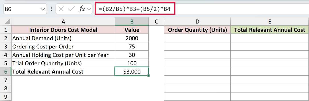
In that formula, B2/B5 is the number of orders per year. Multiplying by B3 gives annual ordering cost. B5/2 is average cycle stock, and multiplying by B4 gives annual holding cost.
At Q=100, annual ordering cost is (2,000/100)×$75=$1,500. Annual holding cost is (100/2)×$30=$1,500, so total relevant annual cost is $3,000.
Here are the steps to build the Data Table:
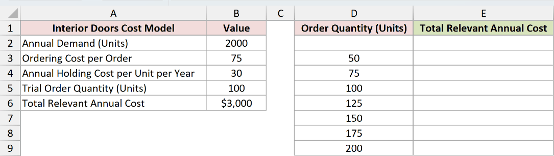
- In a spare column, list the order quantities you want to test. I used 50 up to 200 in steps of 25.
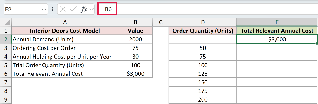
- One row above the first quantity and one column to its right, type a link to the total cost cell (=B6 in my sheet). This is the cell Excel reads down the table.
- Select the block that covers both the quantities and that linking formula. On the Data tab, click What-If Analysis, then choose Data Table.
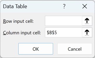
- Leave the Row input cell empty. In the Column input cell box, click the order quantity cell (B5), then click OK.
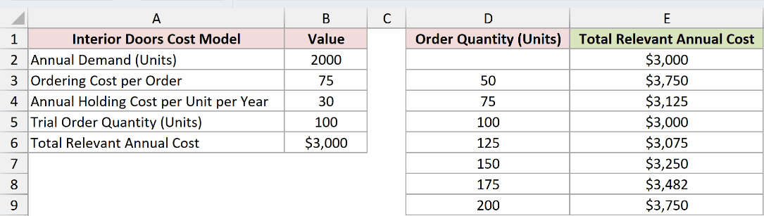
Excel fills in the cost for every listed quantity. It returns 100 exactly because 100 is in the tested list, and its $3,000 cost is the lowest listed result.
If the formula result is not in your list, use smaller increments around the calculated EOQ to compare closer quantities.
Notice the costs barely move on either side of 100. That’s normal. Relevant annual ordering and holding cost is flat near the EOQ, so a nearby practical quantity may cost only slightly more.
Note: The filled results are one linked array, so you can’t edit or delete a single cell inside it. To clear the table, select the whole block of results and delete it together.
Additional Notes About Calculating EOQ in Excel
Here are a few things worth keeping in mind so your EOQ numbers stay reliable.
- Demand and holding cost must use the same period. Ordering cost is per order. Keep currency and stocking units consistent. All inputs must be positive, and holding cost must be greater than zero, or the formula can return misleading errors.
- Carrying rates vary by business. Use a rate that reflects your actual storage, insurance, obsolescence, shrinkage, and capital costs. If you estimate an annual rate, multiply it by unit cost to get annual holding cost per unit.
- When an order must be rounded upward to full packs, use
=CEILING.MATH(calculated_EOQ,pack_size). MROUND rounds to the nearest pack and can round down, so use it only when the nearest pack is acceptable. - The basic EOQ model assumes known, steady demand; constant cost per order and holding cost per unit; no stockouts; no quantity discounts; and replenishment arriving as one lot. With constant lead time, lead time changes the reorder point, not the basic EOQ quantity.
Frequently Asked Questions
What units should the demand and holding cost use?
Demand is units per period, usually per year. Holding cost is currency per stocked unit over that same period. Ordering cost is currency per order, so it does not share the annual or monthly time dimension.
Use the same stocking unit and currency throughout. For an annual model, D is units per year, S is currency per order, H is currency per unit per year, and EOQ is units per order.
Does Excel have a built-in EOQ function?
No. There’s no EOQ or INVENTORY function in Excel. You build it yourself from the SQRT function, which is why the formula in Method #1 is the standard approach. It’s short enough that a dedicated function wouldn’t save you much anyway.
How do I find the reorder point once I know the EOQ?
The EOQ tells you how much to order, not when. With constant lead time and no safety stock, the reorder point is average daily demand times lead time in days. Lead time affects that reorder point, not the basic EOQ quantity.
Do I have to round the EOQ to a whole number?
For full packs, use =CEILING.MATH(calculated_EOQ,pack_size) to round upward. Use MROUND only when the nearest pack, including a lower one, is acceptable. Then compare the practical quantity against the cost model.
Conclusion
In this tutorial, I used =SQRT((2*D*S)/H) for one item and a spilled version for a range. The Data Table then illustrated relevant annual ordering and holding costs for the quantities tested.
The basic EOQ result is a model-based starting point. Keep units and periods consistent, then account separately for omitted costs and supplier pack sizes.
I hope you found this article helpful!
Other Excel articles you may also like:
