
The COUNTA function in Excel counts cells that are not empty.
It includes numbers, text, logical values, errors, and formulas returning an empty string. That last case matters when a cell looks blank but still contains a formula.
In this article, I’ll show you how to count non-empty cells across ranges, check mixed data types, and combine COUNTA with UNIQUE for distinct counts.
COUNTA Function Syntax in Excel
The COUNTA function takes one or more values and returns a count of how many of them are non-empty.
=COUNTA(value1, [value2], ...)
- value1 – the first value or range to count. Required.
- value2, … – additional values or ranges. Optional. You can pass up to 255 arguments in total.
When to Use COUNTA Function
COUNTA shows up any time you need to know how many cells contain anything at all. A few common cases:
- Counting completed survey responses, regardless of whether the response is text or numeric.
- Tracking how many students have submitted an assignment (with blanks meaning “not yet”).
- Checking how many cells in a list have any data, before running a calculation that only makes sense with non-empty values.
- Counting how many rows match a condition by combining COUNTA with FILTER.
- Counting distinct entries in a column by combining COUNTA with UNIQUE.
Example 1: Count Non-Empty Cells in a Range
Let’s start with the most common use of COUNTA: pointing it at a single column and reading the count.
Below is a dataset of ten students in column A with the date each one submitted their assignment in column B. A few cells are blank because those students haven’t submitted yet.
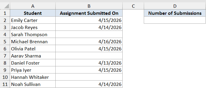
I want to know how many students have submitted, without manually counting the dated rows.
Here is the formula:
=COUNTA(B2:B11)
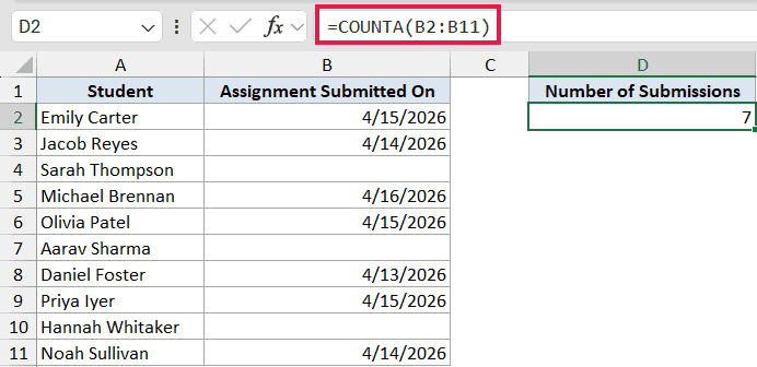
COUNTA walks across B2:B11 and counts every cell that isn’t truly empty. Seven students have a submission date, so the result is 7.
The three blank cells (Sarah, Aarav, and Hannah) are skipped entirely. COUNTA doesn’t care what kind of value is in a cell, only that there is one.
Pro Tip: If you only want to count cells that contain numbers (and skip text and logicals), use COUNT instead of COUNTA. They look almost identical but treat their data very differently.
Example 2: Count Non-Empty Cells Across Multiple Ranges
Here’s a less obvious feature: COUNTA can take up to 255 separate arguments. You don’t have to stick to one continuous range.
Below is a sign-up sheet for two weekend workshops. Saturday signups sit in B2:B7 and Sunday signups sit in B9:B14, with a divider row in between. A few slots are open in each session.
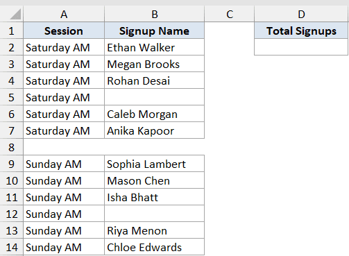
I want a single count of all confirmed signups across both sessions.
Here is the formula:
=COUNTA(B2:B7, B9:B14)
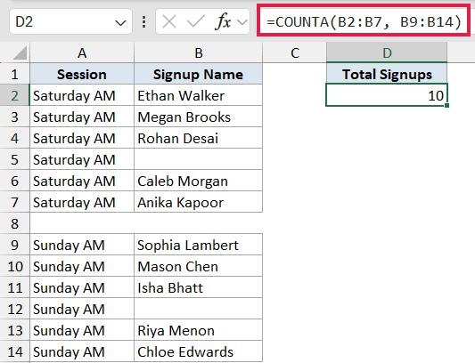
COUNTA takes both ranges as separate arguments and counts the non-empty cells across both. Five Saturday signups plus five Sunday signups gives 10.
The blank cells at B5 and B12 represent open slots, and COUNTA skips them just like it would inside a single range.
This works for any number of ranges. =COUNTA(B2:B7, B9:B14, E2:E20) would happily count three separate blocks at once.
Pro Tip: The ranges don’t have to be the same size, and they don’t even have to be on the same sheet. =COUNTA(Sheet1!A:A, Sheet2!A:A) counts non-empty cells in column A across two whole sheets.
Example 3: COUNTA With Mixed Data Types
This next example catches a lot of people: the difference between “truly empty” and “looks empty”.
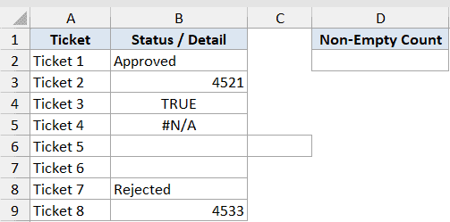
Below is a small ticket queue with eight rows. Each row has a Status / Detail value in column B, but the values are deliberately different kinds: text, a number, a logical, an error, an empty-string formula, and one row that’s actually blank.
I want to count how many of the eight rows have anything in them at all.
Here is the formula:
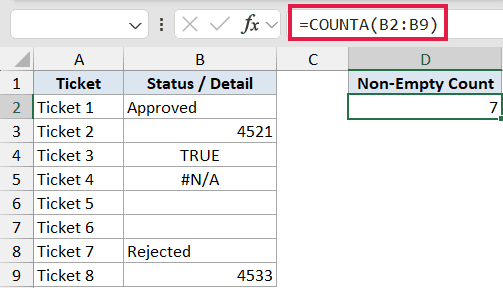
=COUNTA(B2:B9)
How this formula works:
- COUNTA counts the text values (“Approved”, “Rejected”), the numbers (4521, 4533), the logical (TRUE), and the error (#N/A). That’s six.
- Ticket 5 looks empty in the screenshot, but the formula
=IF(C6="","",C6)returns an empty string. To COUNTA, that’s still a value, so it counts. - Ticket 6 is the only truly blank cell. It’s the only one COUNTA skips.
So the total is 7. The cell that visually looks blank (Ticket 5) gets counted, while the cell that actually is blank (Ticket 6) doesn’t.
Pro Tip: Formulas that return "" (empty string) are the most common reason COUNTA returns a higher count than you expect. If you need to skip those too, use SUMPRODUCT instead: =SUMPRODUCT((range<>"")*1).
Example 4: COUNTA Inside FILTER
For the next example, compose COUNTA with FILTER to count just the rows that match a condition.
Below is a customer list with ten rows in column A and each customer’s status in column B (either Active or Inactive).
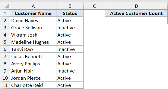
I want a single number telling me how many customers are currently Active, without sorting or filtering the list manually.
Here is the formula:
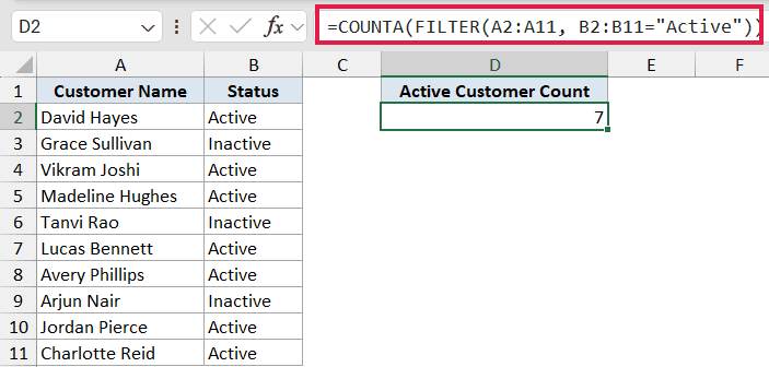
=COUNTA(FILTER(A2:A11, B2:B11="Active"))
How this formula works:
FILTER(A2:A11, B2:B11="Active")returns just the rows whose status is Active, as a spilled array of seven names.COUNTA(...)collapses that spilled array to a single number: 7.
Before dynamic arrays, this kind of conditional count needed COUNTIF (which doesn’t return matching rows) or a SUMPRODUCT trick. With FILTER, the formula reads almost like English.
Pro Tip: This pattern works the other way too. =COUNTA(FILTER(A2:A11, B2:B11="Inactive")) returns 3 here. Swap the condition for any check you need.
Example 5: COUNTA + UNIQUE for a Distinct Count
For the final example, compose COUNTA with UNIQUE to get a count of distinct values in a column.
Below is an order log with fifteen rows. Each row has an Order ID in column A and the region the order shipped to in column B. The same regions repeat across multiple rows.
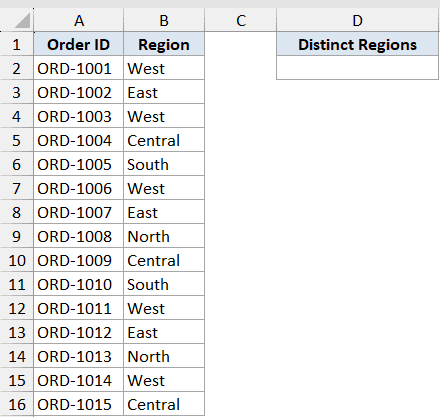
I want to know how many distinct regions the orders shipped to.
Here is the formula:
=COUNTA(UNIQUE(B2:B16))
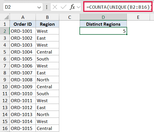
How this formula works:
UNIQUE(B2:B16)returns one entry per distinct region as a spilled array. Out of fifteen rows, only five regions appear: West, East, Central, South, and North.COUNTA(...)reduces that spilled array to its length: 5.
It’s the shortest distinct-count formula in modern Excel, and it works on text, numbers, or a mixed column without changes. For pre-365 alternatives, see the dedicated tutorial on how to count unique values in Excel.
Pro Tip: To count only the regions that appear exactly once in the column, pass TRUE as UNIQUE’s third argument: =COUNTA(UNIQUE(B2:B16, FALSE, TRUE)). With the data above that returns 0, since every region repeats.
Tips & Common Mistakes
- COUNTA and COUNT do different jobs. COUNT only counts cells that contain numbers; COUNTA counts cells that contain anything at all. If a mixed column should return only the numeric count, use COUNT.
- Formulas that return an empty string (
"") are counted as non-empty by COUNTA. If those cells look blank to you but the count seems too high, that’s usually the reason. - A cell with only a space character is also counted. It looks blank but isn’t truly empty.
- Hidden rows still get counted by COUNTA. To count filtered rows only, use
=SUBTOTAL(3, range)instead. SUBTOTAL with function number 3 is “COUNTA on visible cells only”. - COUNTA accepts up to 255 arguments, and the ranges don’t have to be the same size or on the same sheet.
- COUNTA doesn’t spill on its own because it’s a reducer. Compose it with FILTER, UNIQUE, or a spilled range reference like
A2#to bring dynamic-array power into your count.
COUNTA is one of those small, no-frills functions that quietly does a lot of work. It’s perfect for any “how many cells that are not blank” question, and it composes beautifully with FILTER and UNIQUE for more nuanced counts.
Across these five examples, you’ve seen COUNTA on a single range, across multiple ranges, on a mixed-type column with the empty-string gotcha, and combined with FILTER and UNIQUE for conditional and distinct counts.
Related Excel Functions / Articles:
- COUNT Function in Excel
- ISBLANK Function in Excel
- ISTEXT Function in Excel
- How to Count Cells with Text in Excel?
- Count the Number of Yes in Excel (Using COUNTIF)
- Count How Many Times a Word Appears in Excel (Easy Formulas)
- COUNTIF Greater Than Zero in Excel
- How to COUNTIF Partial Match in Excel?
- COUNTIFS Function in Excel
