
Excel’s DEC2HEX function converts a decimal integer into hexadecimal text.
Positive values use the fewest characters needed unless you request leading zeros. Negative values return a fixed 10-character, 40-bit two’s-complement result.
In this article, I’ll show you how to convert decimal values to hexadecimal, add leading zeros, and build RGB color codes.
DEC2HEX Function Syntax in Excel
DEC2HEX has one required argument and one optional argument.
=DEC2HEX(number, [places])
numberis the decimal integer you want to convert. It must be from -549,755,813,888 through 549,755,813,887.placesis the optional result width. DEC2HEX adds leading zeros when a positive result needs fewer characters.
When to Use DEC2HEX Function
- Convert decimal identifiers, register values, or counters into hexadecimal text.
- Create fixed-width hexadecimal codes with leading zeros.
- Build HTML color codes from decimal RGB values.
- Encode negative integers in Excel’s 40-bit two’s-complement format.
- Check whether a value fits DEC2HEX’s signed range.
Example 1: Convert Decimal Values to Hexadecimal
This first example uses a list of telemetry register values.
Below is the dataset with eight decimal values in column A.
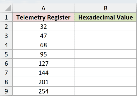
We want one formula in B2 to convert the entire list into hexadecimal text.
Here is the formula:
=DEC2HEX(+A2:A9)
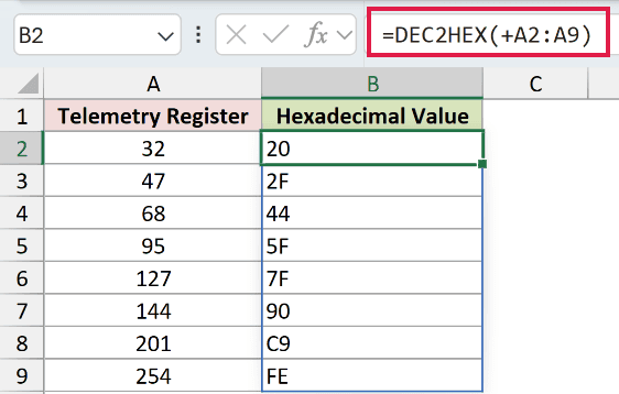
The formula returns 20, 2F, 44, 5F, 7F, 90, C9, and FE.
The leading + passes the source range to DEC2HEX as a value array. The eight results then spill from B2 through B9.
This spilling pattern works in Excel 2021, Excel 2024, Microsoft 365, and Excel for the web.
Pro Tip: Keep the cells below the formula blank. A blocked output range causes a #SPILL! error.
Example 2: Add Leading Zeros to Hex Codes
Fixed-width codes are easier to compare and sort when every result has the same length and retains its leading zeros.
Below is the dataset with equipment numbers in column A.
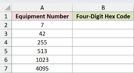
We want every hexadecimal code in B2:B7 to contain four characters.
Here is the formula:
=DEC2HEX(+A2:A7,4)
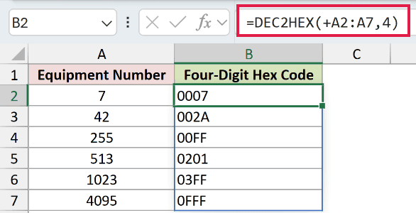
The places argument is 4, so DEC2HEX pads shorter results with zeros on the left.
The values become 0007, 002A, 00FF, 0201, 03FF, and 0FFF.
DEC2HEX returns #NUM! when the requested width is too small for a positive result.
Pro Tip: The result is text, so Excel keeps its leading zeros without a custom number format.
Example 3: Convert RGB Values to Hex Colors
DEC2HEX can convert three RGB channels into a web color code.
Below is the dataset with palette names and decimal red, green, and blue values.
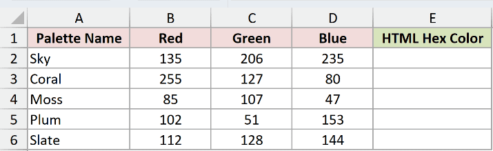
We want to join three two-character hexadecimal values after a hash sign.
Here is the formula:
="#"&DEC2HEX(+B2:B6,2)&DEC2HEX(+C2:C6,2)&DEC2HEX(+D2:D6,2)
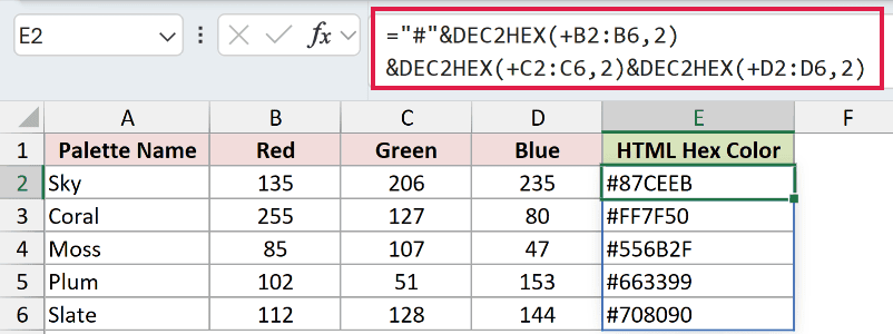
Each DEC2HEX call converts one color channel and pads it to two characters. The ampersands join those parts with #.
The resulting colors are #87CEEB, #FF7F50, #556B2F, #663399, and #708090.
Pro Tip: RGB channels must stay between 0 and 255. Values above 255 need more than two hexadecimal characters.
Example 4: Convert Negative Numbers to Hexadecimal
Negative decimal values use a signed hexadecimal representation.
Below is the dataset with calibration offsets and empty columns for hexadecimal codes and a round-trip check.
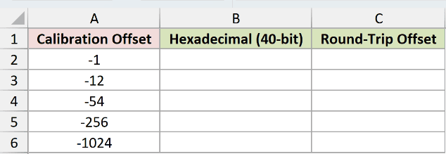
We want DEC2HEX to encode the offsets in B2:B6.
Here is the DEC2HEX formula:
=DEC2HEX(+A2:A6,4)
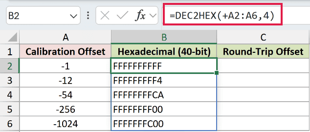
The results are FFFFFFFFFF, FFFFFFFFF4, FFFFFFFFCA, FFFFFFFF00, and FFFFFFFC00.
DEC2HEX ignores places for negative numbers. It always returns 10 characters using 40-bit two’s-complement notation.
We also want to decode each hexadecimal string and confirm the original offset.
Here is the round-trip formula:
=MAP(B2:B6,LAMBDA(code,HEX2DEC(code)))
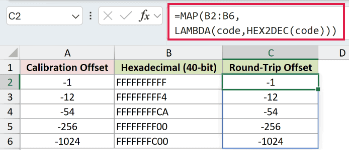
MAP passes each hexadecimal text value to HEX2DEC. The results are -1, -12, -54, -256, and -1024.
MAP is available in Microsoft 365 and Excel 2024. In older versions, apply HEX2DEC to one result per row instead.
Pro Tip: Keep the hexadecimal values as text during the round trip. Letters A through F are valid hexadecimal digits.
Example 5: Convert Larger Numbers With BASE
DEC2HEX supports signed 40-bit integers, which limits its largest positive input.
Below is the dataset with four system counters and empty result columns for DEC2HEX and BASE.
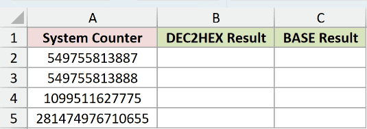
The first test checks each counter against DEC2HEX’s documented range.
Here is the DEC2HEX formula:
=DEC2HEX(+A2:A5)
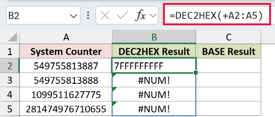
DEC2HEX converts 549755813887 to 7FFFFFFFFF. It returns a #NUM! error for the three larger values.
We also want hexadecimal text for every nonnegative counter in the table.
Here is the BASE formula:
=BASE(A2:A5,16)
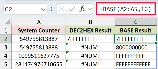
BASE returns 7FFFFFFFFF, 8000000000, FFFFFFFFFF, and FFFFFFFFFFFF.
BASE accepts nonnegative integers below 2^53 and supports bases 2 through 36. It does not create DEC2HEX’s signed representation for negative values.
Pro Tip: Use BASE for a larger nonnegative integer. Use DEC2HEX when you need its signed 40-bit behavior.
Example 6: Troubleshoot DEC2HEX Errors
The number and places arguments can fail for different reasons.
Below is the dataset with seven input and width combinations.
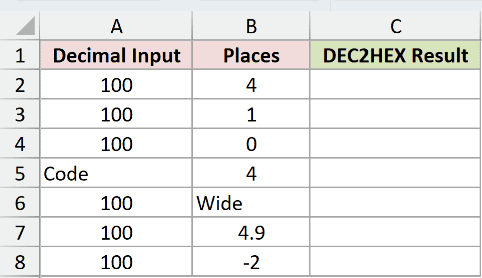
We want to evaluate each row separately so the cause of every result stays visible.
Here is the formula in C2, filled down through C8:
=DEC2HEX(A2,B2)
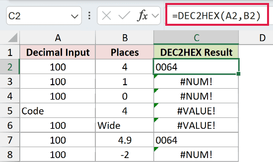
The first row returns 0064 because four places can hold the hexadecimal result for 100.
Rows 3 and 4 return #NUM! because one character and zero characters cannot hold 64. A negative width in row 8 causes the same error.
Text in either argument returns a #VALUE! error, as rows 5 and 6 show. Excel truncates 4.9 to 4 in row 7 and returns 0064.
Pro Tip: Diagnose the argument that failed before using IFERROR. Hiding every error can conceal an out-of-range input or an undersized width.
Tips & Common Mistakes
- Keep
numberfrom -549,755,813,888 through 549,755,813,887. Values outside that range return#NUM!. - Preserve the unary plus in range formulas. It passes the values to DEC2HEX as an array and allows the results to spill.
- Keep the spill range clear in Excel 2021, Excel 2024, Microsoft 365, and Excel for the web.
- Remember that negative values always return 10 hexadecimal characters. DEC2HEX ignores
placesfor those inputs. - Use enough places for a positive result. Excel truncates fractional places, while zero, negative, or insufficient places return
#NUM!. - Treat DEC2HEX output as text. This preserves hexadecimal letters and any leading zeros.
I covered range conversion, fixed-width codes, RGB colors, negative values, larger counters, and common DEC2HEX errors.
I also compared DEC2HEX with HEX2DEC and BASE. I hope you found this article helpful.
Related Excel Functions / Articles:
