
Excel’s DGET function extracts one value from a database record that matches a worksheet criteria range.
It is useful when field headings and conditions in cells define the record you need. You can combine conditions without embedding each one directly in the formula.
Exactly one record must match. DGET returns an error when no record qualifies or when multiple records meet the criteria.
In this article, I’ll show you how to retrieve records using multiple criteria, require an exact text match, and handle unsuccessful lookups.
DGET Function Syntax in Excel
The DGET function returns one value from the field and record that meet your criteria.
=DGET(database,field,criteria)
- database (required) is the complete list, including the header row. Each row is a record, and each column is a field.
- field (required) identifies the column to return. Use its header in quotes, a cell containing that header, or its position within the database.
- criteria (required) is a worksheet range containing at least one matching database header and a condition beneath it.
When to Use DGET Function
- Return one field from a record identified by an editable criteria cell.
- Use two or more conditions together without building them into the formula.
- Find the only record above or below a specified limit.
- Make duplicate or missing matches visible through the built-in #NUM! and #VALUE! errors.
Example 1: Look Up One Employee’s Sales
Let’s start with a straightforward employee lookup.
Below is the dataset. Columns A to F hold the sales records, while column H contains the employee criterion and column J holds the result.
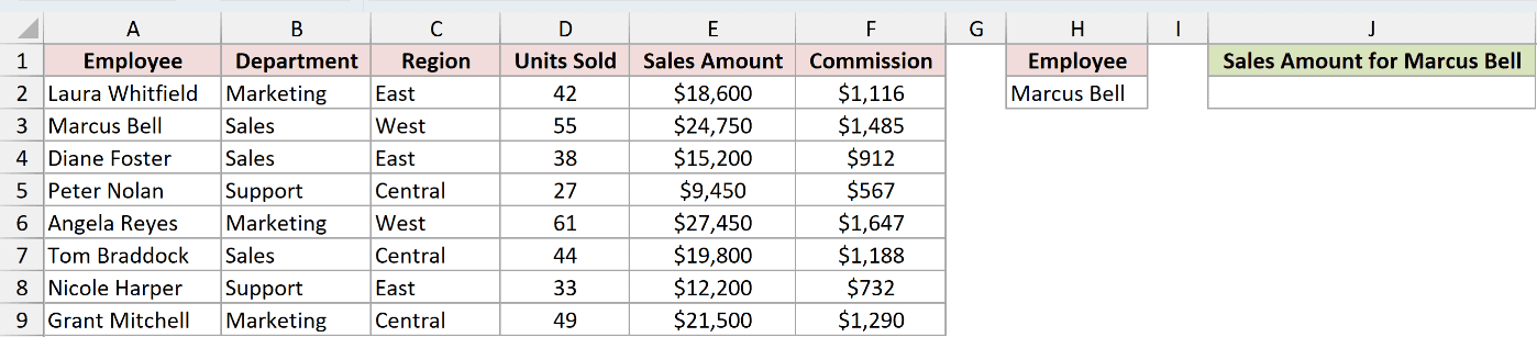
We want to return the Sales Amount for Marcus Bell.
Here is the formula:
=DGET(A1:F9,"Sales Amount",H1:H2)
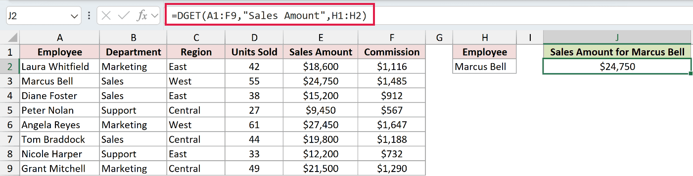
The database includes its headers in A1:F9. The field argument tells DGET to return a value from the Sales Amount column.
The criteria range H1:H2 contains the matching Employee header and Marcus Bell. One record qualifies, so DGET returns $24,750.
Changing H2 gives you another lookup without editing the formula. That makes DGET useful when a worksheet has a dashboard-style input cell.
For a single-value lookup, XLOOKUP is more direct and does not need a separate criteria header. DGET remains useful when you want conditions visible in worksheet cells.
Example 2: Use DGET With Multiple Criteria
Now let’s see what happens when one condition is not specific enough.
Below is the dataset. Columns A to E list sales activity, columns G and H form the criteria block, and columns J and K show both results.
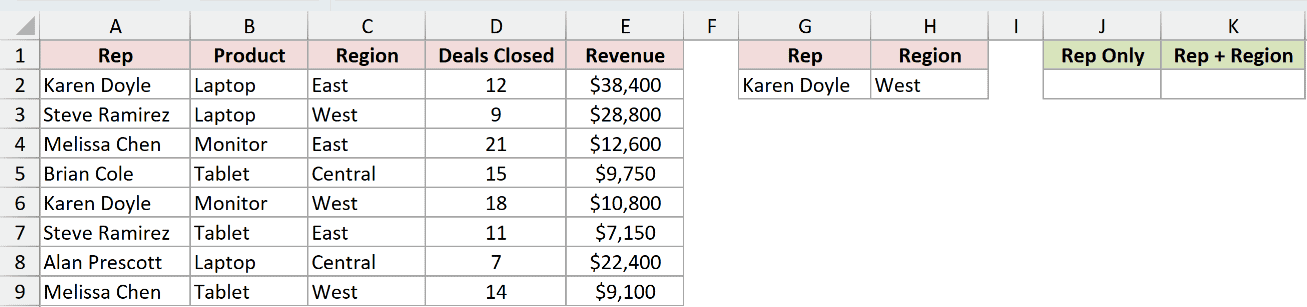
We want Karen Doyle’s West region revenue, but we’ll first try her name alone.
Here is the formula using only the Rep criterion:
=DGET(A1:E9,"Revenue",G1:G2)
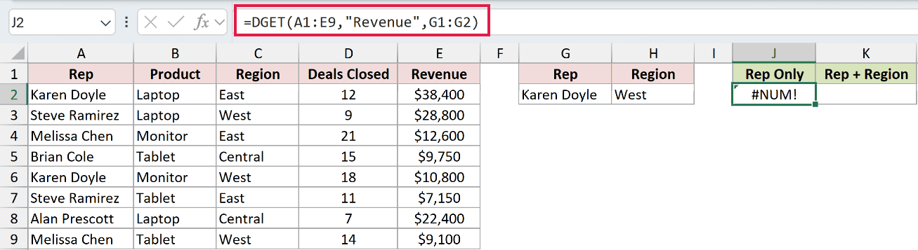
The formula returns #NUM! because Karen Doyle has two records. DGET will not choose one when more than one record meets the criteria.
Here is the formula using both Rep and Region:
=DGET(A1:E9,"Revenue",G1:H2)
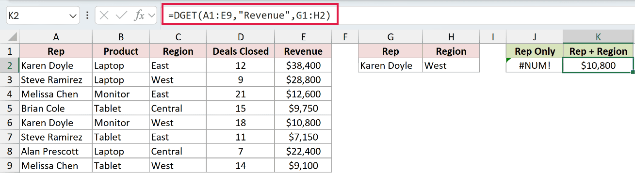
Placing Karen Doyle and West on the same criteria row joins them with AND. Only one record now qualifies, so the result is $10,800.
Both formulas use the same criteria block. The only change is widening the criteria argument from G1:G2 to G1:H2.
Example 3: Use a Comparison Operator in DGET
Here’s a useful way to look up a record that crosses a limit.
Below is the dataset. Columns A to E contain project details, column G holds the budget criterion, and columns I and J compare two field forms.
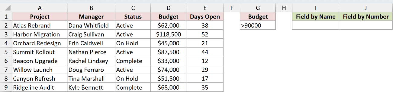
We want the manager of the only project with a budget above $90,000.
Here is the formula with the field supplied by name:
=DGET(A1:E9,"Manager",G1:G2)
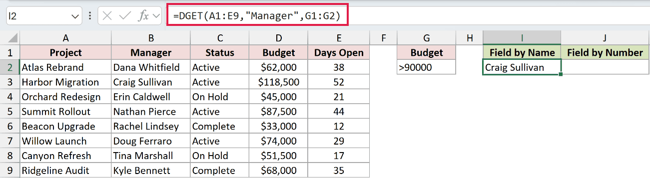
The criteria value in G2 is >90000. Excel reads the comparison operator and finds Harbor Migration, whose $118,500 budget is the only qualifying value.
DGET then returns Craig Sullivan from the Manager field.
Here is the equivalent formula with the field supplied by position:
=DGET(A1:E9,2,G1:G2)
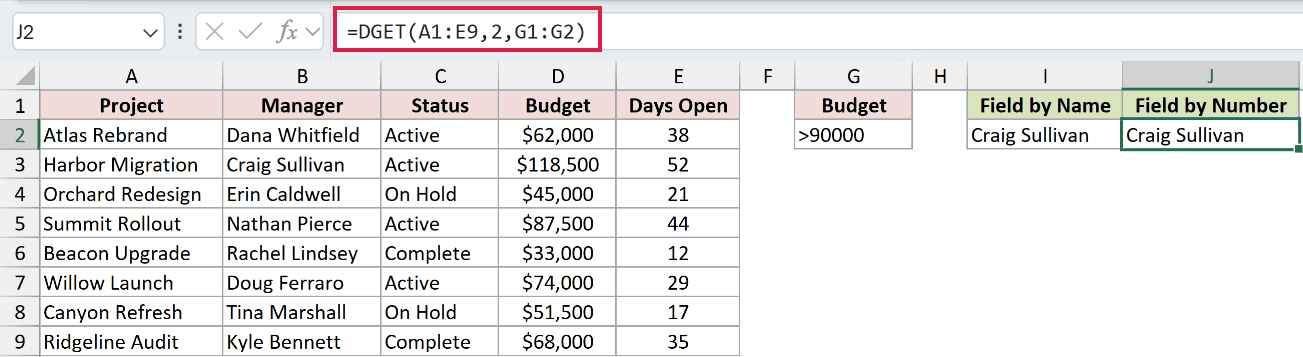
The number 2 means the second column within A1:E9. That is the Manager column, so this formula also returns Craig Sullivan.
Example 4: Handle DGET #VALUE! With IFERROR
Next, let’s handle a criterion that matches no record.
Below is the dataset. Columns A to E contain the product catalog, column G holds the requested SKU, and columns I and J show both outcomes.
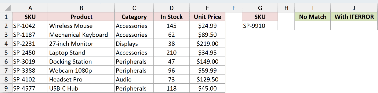
We want the Unit Price for SKU SP-9910, which is not in the catalog.
Here is the unguarded DGET formula:
=DGET(A1:E9,"Unit Price",G1:G2)
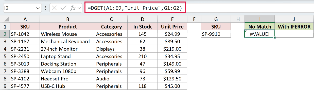
The formula returns #VALUE! because no record has that SKU. This error is DGET’s normal response to a missing match.
Here is the formula wrapped in IFERROR:
=IFERROR(DGET(A1:E9,"Unit Price",G1:G2),"Not found")
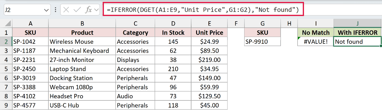
IFERROR replaces the error with Not found, which is easier to read on a report.
Pro Tip: IFERROR catches every error from DGET. A “Not found” message can therefore hide a #NUM! duplicate as well as a genuine #VALUE! no-match.
Example 5: Force an Exact DGET Text Match
This example covers a text-matching rule that can catch you out.
Below is the dataset. Columns A to E list subscriptions, columns G and I hold two Plan criteria, and columns K and L show the results.
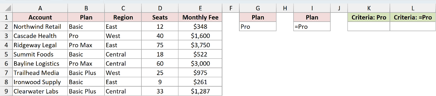
We want the Monthly Fee for the record whose Plan is exactly Pro.
Here is the formula using Pro as the criterion:
=DGET(A1:E9,"Monthly Fee",G1:G2)
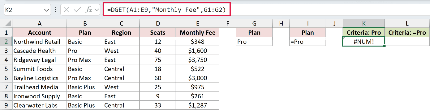
The formula returns #NUM! because DGET treats text criteria as begins-with matches. Pro matches the Pro record and both Pro Max records.
Cell I2 displays =Pro, which forces an exact text match. The cell stores this criteria value through ="=Pro", but it is not another result formula.
Here is the formula using that exact-match criteria range:
=DGET(A1:E9,"Monthly Fee",I1:I2)
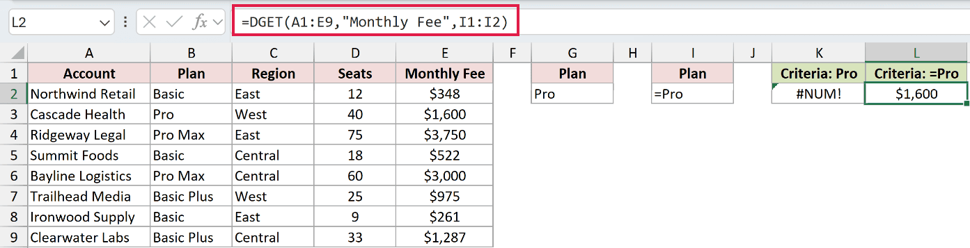
Only the Cascade Health record now qualifies, so DGET returns $1,600.
XLOOKUP matches exactly by default, so it avoids this begins-with trap. DGET needs the special criteria value when text prefixes overlap.
Example 6: Return a Value From the Left
Finally, let’s return a field that sits before the criteria column.
Below is the dataset. Columns A to E hold invoice records, column G contains the Days Outstanding criterion, and column I holds the matching client.
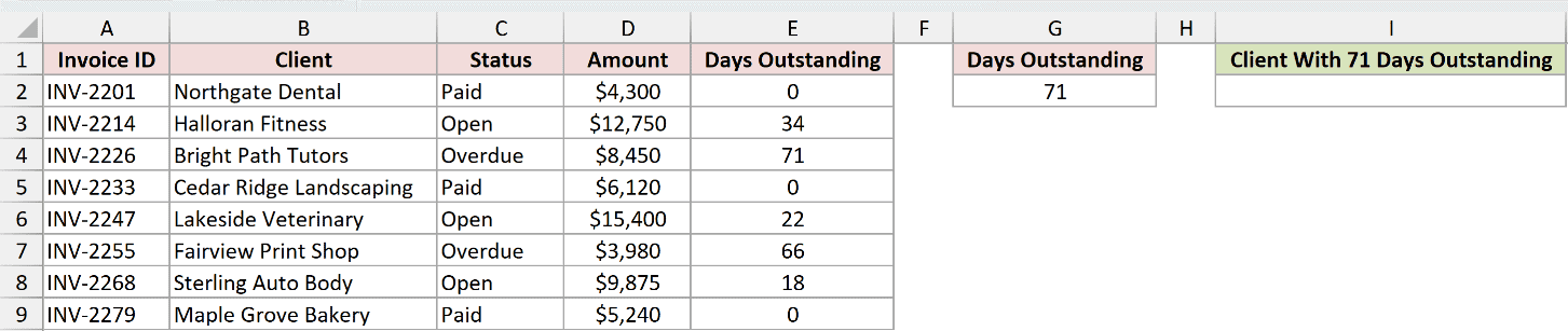
We want the client whose invoice has exactly 71 days outstanding.
Here is the formula:
=DGET(A1:E9,"Client",G1:G2)
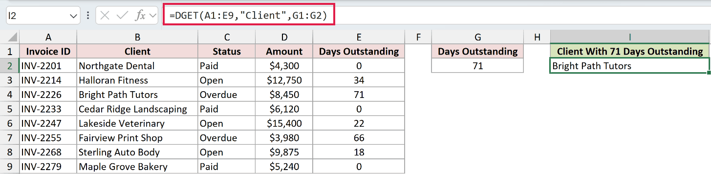
DGET checks Days Outstanding in column E and returns Bright Path Tutors from column B. The return column can sit to the left of the criteria column.
For this lookup, XLOOKUP uses =XLOOKUP(G2,E2:E9,B2:B9). It can look left as easily as right and works better when you need to copy lookups down a column.
Tips & Common Mistakes
- Include the database header row in the first argument. A headerless range prevents DGET from identifying its fields correctly.
- Keep the criteria block beside the list, to its right. A new record belongs in the first row below the list and could collide with criteria parked there.
- Make each criteria header match its database header. The comparison is case-insensitive, but the wording still needs to match.
- Text criteria use begins-with matching and ignore case. Wildcards also work, with an asterisk matching any run of characters and a question mark matching one character.
- A blank criteria cell matches every record. That often produces #NUM! because several records qualify.
- Conditions on one criteria row use AND. Separate criteria rows use OR, which often creates multiple matches and leads to #NUM!.
- DGET returns #VALUE! when no record matches and #NUM! when several records match. A missing field header can also produce #VALUE!.
- One DGET lookup needs one headed criteria block. The function does not spill, and copying it down can shift the criteria range away from its header.
- Use FILTER when you want every matching record.
DGET is best when you expect one record and want Excel to flag missing or duplicate matches instead of choosing for you.
Its criteria pattern also carries across to DSUM, DCOUNT, DAVERAGE, DMAX, and DMIN.
Related Excel Functions / Articles:
