
If you want to pull a value out of a table in Excel, you now have two functions for the job, and it is not obvious which one you should reach for.
VLOOKUP has been the standard answer for over twenty years, and XLOOKUP is the newer function Microsoft built to replace it.
Once you see the two running side by side on the same data, though, the choice gets easy.
In this article I’ll compare XLOOKUP and VLOOKUP across seven examples, and show you exactly where the older function lets you down.
Note: XLOOKUP is available in Excel 2021, Excel 2024, Excel for Microsoft 365, and Excel for the web. VLOOKUP works in every version of Excel.
VLOOKUP Function
VLOOKUP searches for your value in the first column of a range, then returns a value from one of the columns to the right of it, in the same row.
It has shipped with every version of Excel, which is why it turns up in almost every workbook that has ever been passed around an office.
Here is the syntax and what each part does.
| Part | What it means |
|---|---|
| Syntax | VLOOKUP(lookup_value, table_array, col_index_num, [range_lookup]) |
| lookup_value | The value you are searching for. |
| table_array | The range to search. VLOOKUP looks in its first column only. |
| col_index_num | Which column of that range to return, counted from the left. |
| [range_lookup] | FALSE for an exact match. TRUE or omitted for an approximate match. |
XLOOKUP Function
XLOOKUP searches one range for your value and returns the matching item from a second, separate range. Those two ranges can sit anywhere, in any order.
It matches exactly by default, it has its own argument for what to show when nothing is found, and it can hand back more than one column at a time.
XLOOKUP is a dynamic array function. When the return range is wider than one column, the results spill into the neighboring cells on their own.
| Part | What it means |
|---|---|
| Syntax | XLOOKUP(lookup_value, lookup_array, return_array, [if_not_found], [match_mode], [search_mode]) |
| lookup_value | The value you are searching for. |
| lookup_array | The range to search in. |
| return_array | The range to return the answer from. |
| [if_not_found] | What to show when there is no match. Defaults to #N/A. |
| [match_mode] | 0 exact (default), -1 next smaller, 1 next larger, 2 wildcards. |
| [search_mode] | 1 top to bottom (default), -1 bottom to top, 2 or -2 binary search. |
XLOOKUP vs VLOOKUP: Side-by-Side Examples
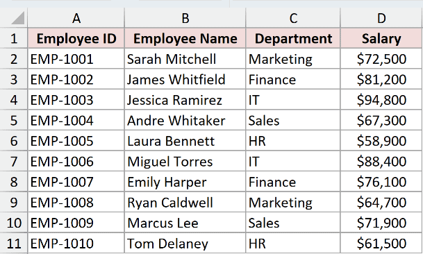
Below I have an employee table in A1:D11. Each example uses this data, with the layout adjusted where the example needs it.
Example #1: Performing a Basic Lookup
From the employee table, I want the salary for the employee name sitting in cell F2, which is Jessica Ramirez.
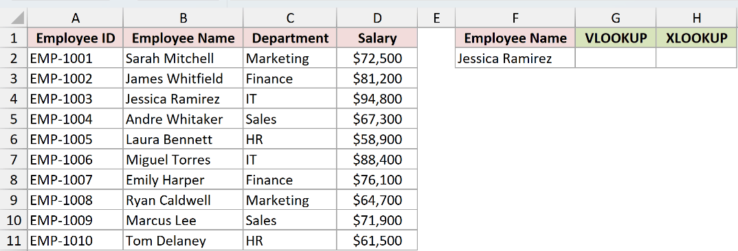
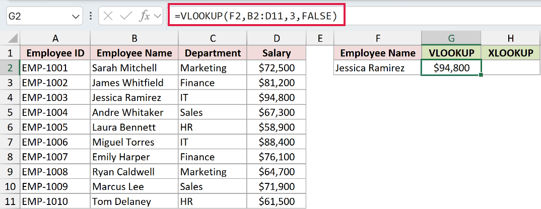
Here is the VLOOKUP formula:
=VLOOKUP(F2,B2:D11,3,FALSE)
And here is the XLOOKUP formula:
=XLOOKUP(F2,B2:B11,D2:D11)
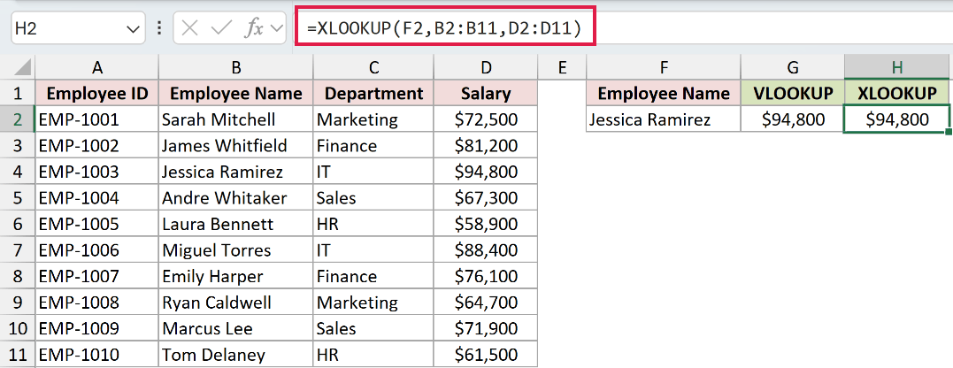
Both return 94800.
VLOOKUP searches B2:D11, finds Jessica Ramirez in the first column of that range, then counts three columns across and returns what is sitting there. FALSE at the end is what forces an exact match.
XLOOKUP asks for two ranges instead of a count. B2:B11 is where to look, D2:D11 is what to return. Nothing to count, and exact match is already the default.
Same answer either way. XLOOKUP just says what it is doing instead of making you count columns.
Example #2: Looking Up to the Left
Same employee table, but this time I want the Employee ID for the name in F2. The IDs sit in column A, to the left of the names.
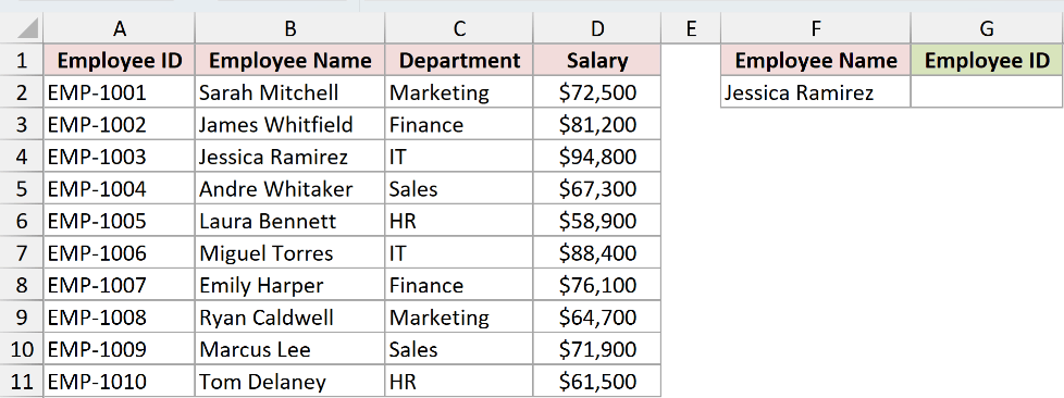
VLOOKUP cannot do this with B2:D11. It searches the first column of the range you give it and returns columns to the right, and there is nothing to the right that holds an ID.
Widening the range to A2:D11 does not rescue it either. VLOOKUP would then be searching column A for a name, and the names are in column B.
The usual workarounds are switching to INDEX MATCH, or physically moving the ID column so it sits to the right of the names.
XLOOKUP has no such limit:
=XLOOKUP(F2,B2:B11,A2:A11)
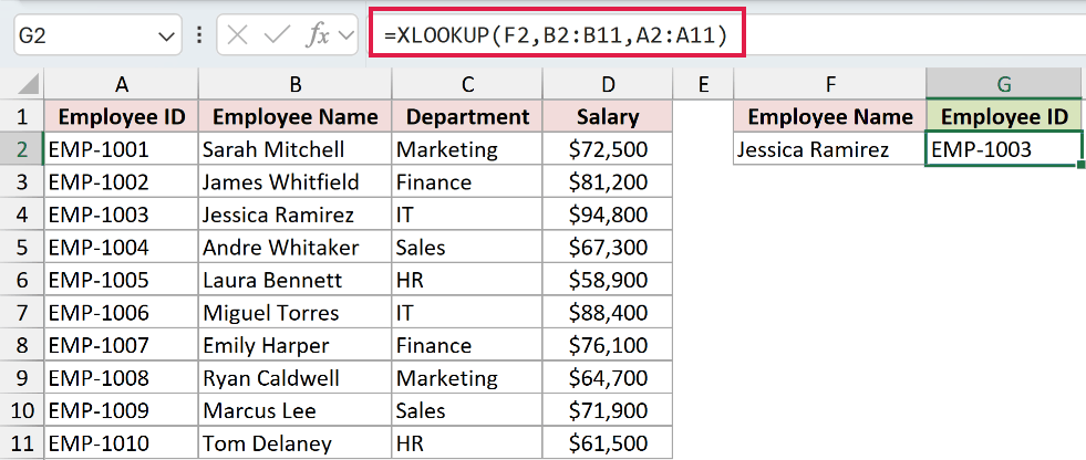
It returns EMP-1003. The lookup range is column B, the return range is column A, and XLOOKUP does not care that one sits to the left of the other.
Left lookups are the classic VLOOKUP wall. XLOOKUP does not have one.
Example #3: Exact Match vs Approximate Match Defaults
Same employee table, same goal as Example #1, with one change. The name in F2 is “Emily Harpar”, a misspelling of Emily Harper, and I am leaving VLOOKUP’s fourth argument off.
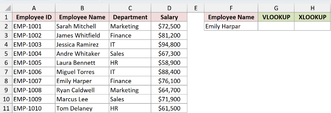
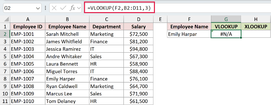
Here is the VLOOKUP formula with no fourth argument:
=VLOOKUP(F2,B2:D11,3)
And the XLOOKUP formula, also with its optional arguments left off:
=XLOOKUP(F2,B2:B11,D2:D11)
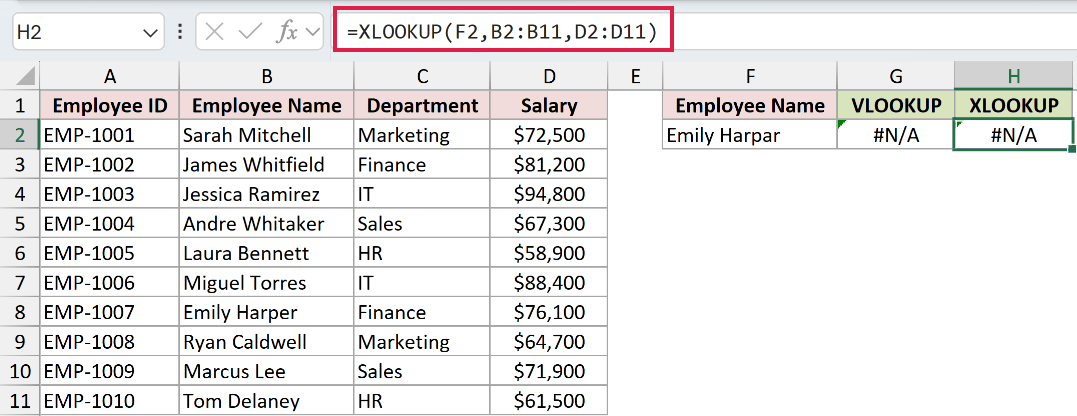
Leaving the fourth argument off puts VLOOKUP into approximate match. That is its default, and it is almost never what you want when you are looking up a name.
Approximate match returns the largest value that is less than or equal to what you searched for, and it only behaves if the lookup column is sorted in ascending order.
This table is sorted by Employee ID, not by name. The requirement is not met, so whatever comes back from that formula is not a real answer.
On my table it happens to land on #N/A. That is luck, not safety. Point the same default at different unsorted data and it can return a real-looking salary that belongs to someone else, with no error anywhere.
XLOOKUP defaults to an exact match. “Emily Harpar” is not in the list, so it returns #N/A every time, which is the truthful answer to the question I asked.
To be fair to VLOOKUP, it does not always need sorted data. That requirement belongs to approximate match only. Add FALSE as the fourth argument and it matches exactly on data in any order.
VLOOKUP’s default is the dangerous one. XLOOKUP’s default is the safe one.
Example #4: Handling Missing Values
Same employee table. This time F2 holds “John Carter”, who does not work here, and I want the cell to say “Not found” instead of throwing an error at the reader.
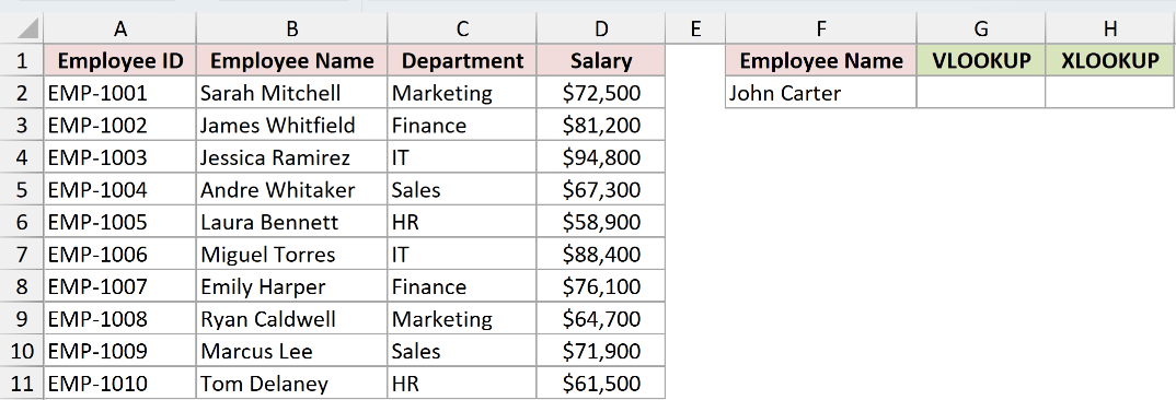
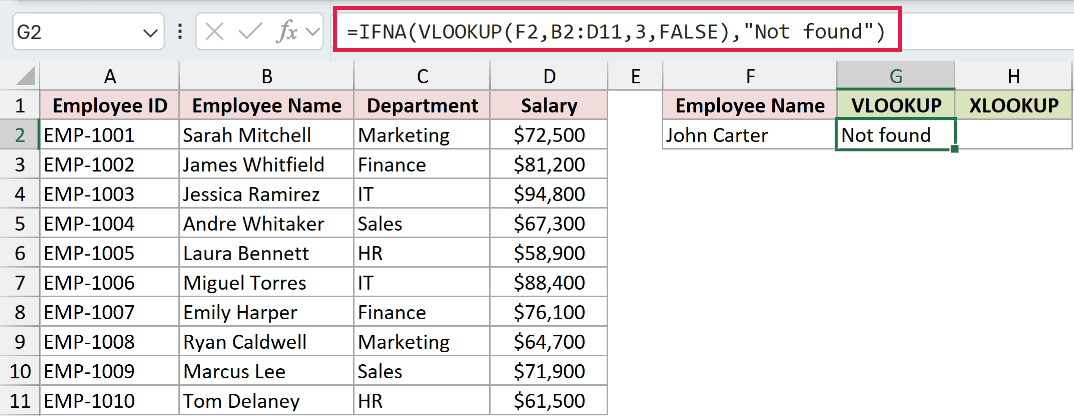
With VLOOKUP, you wrap the whole formula in IFNA:
=IFNA(VLOOKUP(F2,B2:D11,3,FALSE),"Not found")
With XLOOKUP, it is the fourth argument:
=XLOOKUP(F2,B2:B11,D2:D11,"Not found")
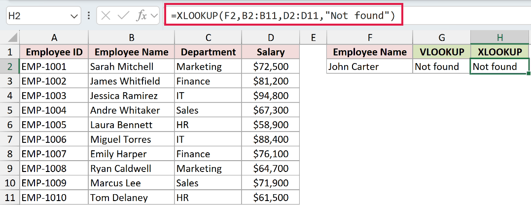
Both cells end up showing “Not found”. The difference is what it took to get there.
VLOOKUP on its own returns #N/A when the name is missing, so you need a second function sitting around the first one just to change what the reader sees.
XLOOKUP has the same idea built into its syntax. The if_not_found argument is the fourth slot, and it takes any text you want.
Reach for IFNA rather than IFERROR on that wrapper. IFERROR swallows every error type, so a genuinely broken formula would also come back as “Not found” and you would never spot it.
One argument against one extra function wrapped around the whole formula.
Example #5: Returning Multiple Columns
Same employee table. F2 holds “Miguel Torres”, and I want both his department and his salary, not just one of them.
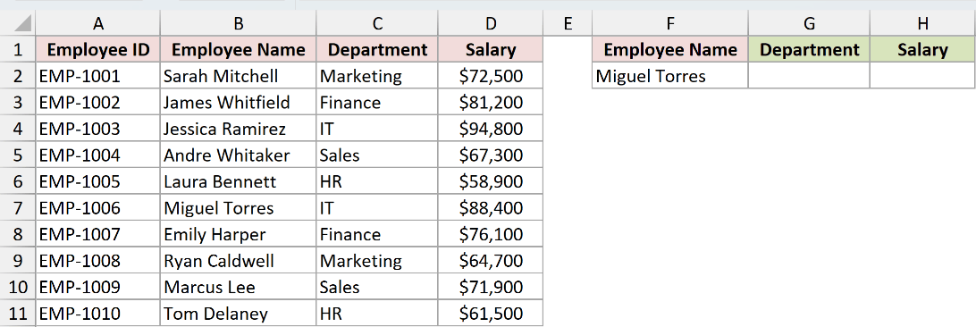
VLOOKUP needs one formula per column. Here is the one for the department:
=VLOOKUP(F2,B2:D11,2,FALSE)
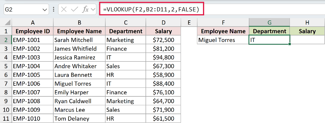
And here is the one for the salary:
=VLOOKUP(F2,B2:D11,3,FALSE)
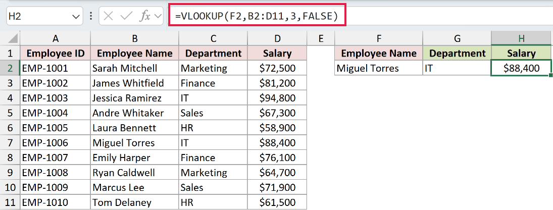
XLOOKUP does both in a single formula:
=XLOOKUP(F2,B2:B11,C2:D11)
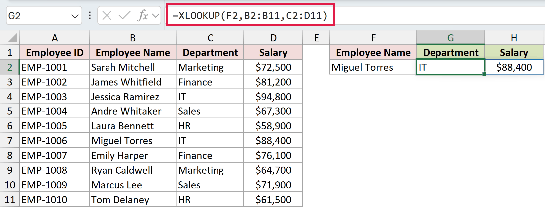
The return range C2:D11 is two columns wide, so the formula spills its results across G2 and H2 automatically. You type it once in G2 and Excel fills H2 for you.
The answers are IT and 88400, and they came from one formula that never mentions a column number.
The VLOOKUP pair gets you to the same place, but you now have two formulas to keep in step and two hard-coded numbers to maintain.
One thing to watch with the spill. If H2 already has something in it, XLOOKUP returns #SPILL! rather than overwriting your data.
One formula that spills, against two formulas and two column counts to keep straight.
Example #6: Searching From the Bottom
Same employee table. F2 holds the department “IT”, and I want the name of the last employee listed in that department, not the first one.
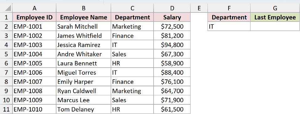
Two people are in IT here. Jessica Ramirez in row 4 and Miguel Torres in row 7. A plain lookup returns the first one it hits, so it would give me Jessica Ramirez.
VLOOKUP has no way to change that. It scans top to bottom and stops at the first match, and there is no argument that reverses it.
XLOOKUP has one:
=XLOOKUP(F2,C2:C11,B2:B11,,0,-1)
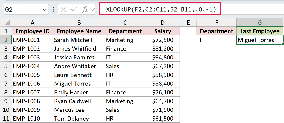
The result is Miguel Torres, the last IT row in the table.
The two trailing arguments do the work. 0 is match_mode, asking for an exact match. -1 is search_mode, telling XLOOKUP to start at the bottom and work upwards.
The gap between the two commas is the if_not_found slot. I skipped past it because the two arguments I actually need sit behind it in the syntax.
Reverse search is a single argument in XLOOKUP. VLOOKUP has no version of it.
Example #7: Inserting or Deleting Columns
Same employee table, same basic salary lookup from Example #1. Now say someone inserts a new column between Employee Name and Department, maybe to hold an email address.
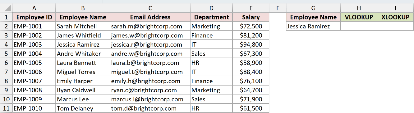
Nothing about the data is wrong. A field got added, which is the most ordinary thing that can happen to a spreadsheet.
Salary moves from column D to column E. Both formulas update their ranges by themselves, because Excel adjusts references when you insert inside them. The lookup cell slides over the same way, from F2 to G2.
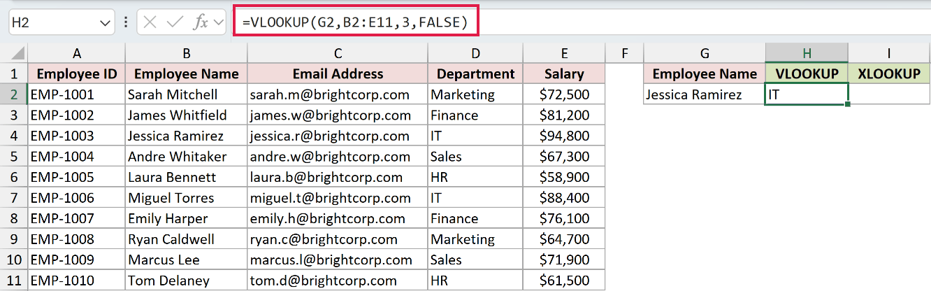
The VLOOKUP formula becomes this:
=VLOOKUP(G2,B2:E11,3,FALSE)
And the XLOOKUP formula becomes this:
=XLOOKUP(G2,B2:B11,E2:E11)
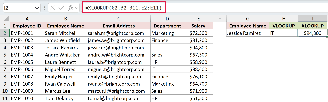
Look at what happened to the 3. The range grew to B2:E11, but the column number stayed put, and it had to. It is a plain number typed into the formula.
Column 3 of B2:E11 is now the Department column. So a formula that used to return 94800 quietly starts returning IT instead.
XLOOKUP had no column number to go stale. It pointed at the salary range itself, that range shifted to E2:E11, and the reference shifted with it.
This is a risky failure because the formula still returns a plausible value and never shows an error.
Reading about a formula going wrong is one thing. Breaking it yourself is better. Click through the scenarios below and watch how each function reacts.
Lookup stress test: VLOOKUP vs XLOOKUP
Same dataset, different lookup problems. Pick a scenario and watch how each formula responds.
XLOOKUP vs VLOOKUP: Summary Table
| Compared on | VLOOKUP | XLOOKUP |
|---|---|---|
| Availability | Every version of Excel | Excel 2021, Excel 2024, Microsoft 365, Excel for the web |
| Lookup direction | Return column must sit to the right | Any direction, left or right |
| Default match | Approximate | Exact |
| Missing values | #N/A unless you wrap it in IFNA | Built-in if_not_found argument |
| Multiple columns | One formula per column | Spills a whole block from one formula |
| Search direction | Top to bottom only | Top to bottom or bottom to top |
| Insert or delete a column | An inserted column can return the wrong field; a deleted return column can produce #REF! | Lookup and return ranges adjust with the sheet |
| Wildcards | Work by default in exact-match mode | Need match_mode set to 2 |
| Syntax | 4 arguments, one of them a column count | 6 arguments, 3 of them optional |
Which One Should You Use?
Use XLOOKUP if your version of Excel has it. For most people that is the whole answer.
It is safer by default, it reads better six months later, and it does not fall apart when a colleague adds a column to your sheet.
VLOOKUP is the fallback, not the first pick. Reach for it when you are on Excel 2019 or older, or when the file is going to someone who is.
That compatibility gap is real. An XLOOKUP formula opened in an older version returns #NAME?, so VLOOKUP still earns its place in shared files.
Frequently Asked Questions
Is XLOOKUP faster than VLOOKUP?
On ordinary worksheets, both are usually fast enough that speed should not decide the choice. XLOOKUP also supports binary-search modes for sorted data, but Microsoft warns that they can return invalid results when the lookup array is not sorted correctly. Test with your own workbook if performance matters.
Can XLOOKUP completely replace VLOOKUP?
For anything VLOOKUP actually does, yes. The only thing keeping VLOOKUP alive is Excel versions that do not have XLOOKUP yet.
Why is XLOOKUP not showing in my Excel?
Your version does not include it. XLOOKUP needs Excel 2021, Excel 2024, Microsoft 365, or Excel for the web. On Excel 2019 and older it will not appear, and a file that uses it shows #NAME? instead.
Does XLOOKUP work with wildcards?
Yes, but you have to ask for it. Set match_mode to 2 and then * and ? work as wildcards. VLOOKUP treats them as wildcards by default when you are doing an exact match.
Conclusion
I compared XLOOKUP and VLOOKUP across seven common lookup tasks. The examples show why XLOOKUP is easier to read and less fragile, while VLOOKUP remains useful for files that must work in older Excel versions.
I hope you found this article helpful.
Other Excel articles you may also like:
- XMATCH Function in Excel
- LOOKUP Function in Excel
- How to Use VLOOKUP with Multiple Criteria in Excel
- VLOOKUP Not Working – 7 Possible Reasons + Fix!
- Bulk Find and Replace in Excel
- COLUMN function
- COLUMNS function
- Excel FALSE function
- Match names with spelling differences in Excel
- How to VLOOKUP From Another Sheet
