MAKEARRAY Function in Excel

If you want to build a calculated grid without filling every cell by hand, MAKEARRAY gives each output cell its own row and column position.

In this article, I’ll show you how to use those positions for tables, codes, comparisons, projections, and percentage grids.

MAKEARRAY is a dynamic array function. It spills a whole block of results into the cells below and to the right.

It is available in Microsoft 365, Excel 2024, and Excel for the web. Earlier versions return #NAME?, with no legacy array-formula fallback.

MAKEARRAY Function Syntax in Excel

MAKEARRAY needs the size of the new array and a LAMBDA that calculates each cell.

=MAKEARRAY(rows,cols,lambda(row,col))

• rows (required) is the number of rows to create. It must be greater than zero.
• cols (required) is the number of columns to create. It must be greater than zero.
• lambda (required) calculates each result using two parameters, first the row position and then the column position.

Both positions start at 1 inside the new array. They are not worksheet row and column numbers.

When to Use MAKEARRAY Function

• Build a two-way grid where every result depends on its row and column.
• Replace a two-variable What-If Data Table with a formula that updates normally.
• Generate labels or codes across a block of positions.
• Calculate each value against the total for its own row or column.
• Handle a position-based calculation that MAP cannot perform from values alone.

For a plain list or evenly stepped grid, use SEQUENCE instead. MAKEARRAY is usually more work than you need for that job.

Example 1: Build a Multiplication Table

Let’s start with a grid that makes the row and column positions easy to see.

Below is the dataset. The numbers 1 through 9 run across row 1 and down column A.

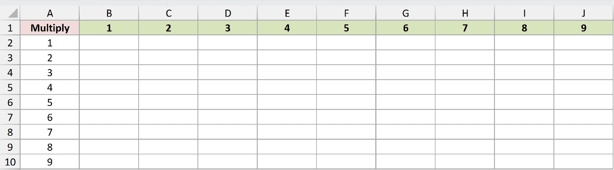
We want one formula in B2 to build the full 9 by 9 multiplication table.

Here is the formula:

=MAKEARRAY(9,9,LAMBDA(r,c,r*c))

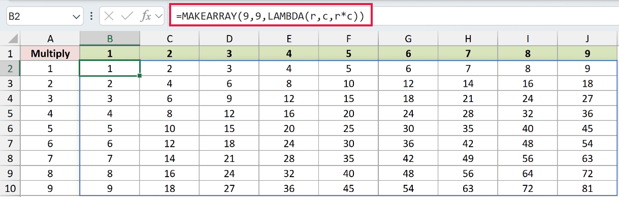
Excel calls the LAMBDA once for each of the 81 cells. It multiplies each cell’s row position by its column position.

That gives 1 in B2, 18 in J3, and 81 in J10.

For this table, =SEQUENCE(9)*SEQUENCE(1,9) is shorter. MAKEARRAY still makes the two positions easy to see.

Pro Tip: The names r and c are your choice. Their order matters because the first parameter receives the row position and the second receives the column position.

Example 2: Create a Commission Grid

Now let’s use row and column positions to pull inputs from two separate lists.

Below is the dataset. Column A lists eight affiliates, column B contains referred sales, and C1:F1 holds four commission rates.

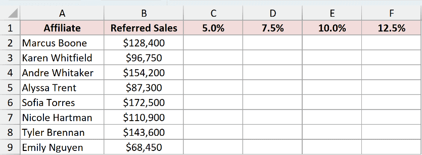
We want to calculate the commission for every affiliate and rate combination.

Here is the formula:

=MAKEARRAY(8,4,LAMBDA(r,c,INDEX($B$2:$B$9,r)*INDEX($C$1:$F$1,c)))

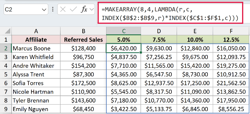
The first INDEX uses r to fetch an affiliate’s sales. The second uses c to fetch the rate at the top of that result column.

Marcus Boone’s $128,400 produces $6,420.00 at 5% and $16,050.00 at 12.5%. Emily Nguyen’s 12.5% commission is $8,556.25.

MAKEARRAY is easier to extend when the calculation also needs lookups, tests, or other per-cell logic. For this grid, =B2:B9*C1:F1 is the shorter option.

Example 3: Generate Warehouse Bin Codes

Here’s a text example, since MAKEARRAY is not limited to numbers.

Below is the dataset. Column A contains aisle letters A through F, and row 1 names four bin positions.

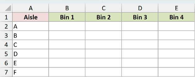
We want to create one code for every aisle and bin combination.

Here is the formula:

=MAKEARRAY(6,4,LAMBDA(r,c,INDEX($A$2:$A$7,r)&"-"&TEXT(c,"00")))

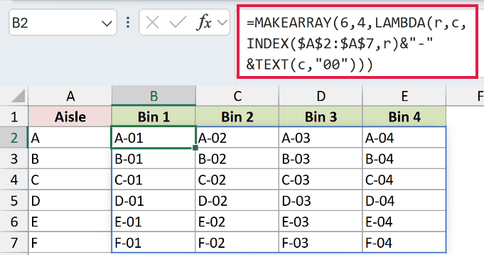
INDEX uses the row position to retrieve the aisle letter. TEXT formats the column position with two digits before joining both parts.

The spilled block starts with A-01 and ends with F-04. The leading zero keeps every bin number the same width.

Pro Tip: MAKEARRAY cannot read the cells it spills into. Pull worksheet values into the LAMBDA with INDEX or another lookup function.

Example 4: Compare Hours With Certification Levels

Let’s add an IF test inside the LAMBDA.

Below is the dataset. Columns A and B list six technicians and their training hours. C1:F1 holds certification thresholds of 20, 40, 60, and 80 hours.

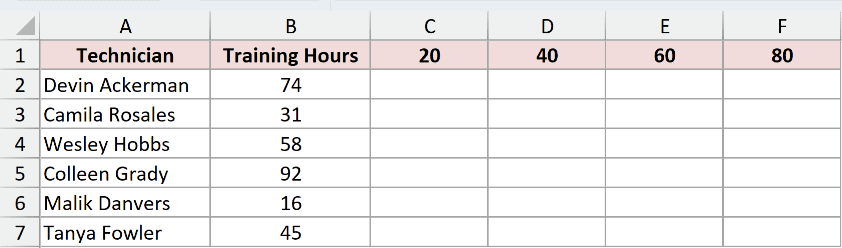
We want each result to show whether a technician has cleared that certification level.

Here is the formula:

=MAKEARRAY(6,4,LAMBDA(r,c,IF(INDEX($B$2:$B$7,r)>=INDEX($C$1:$F$1,c),"Yes","No")))

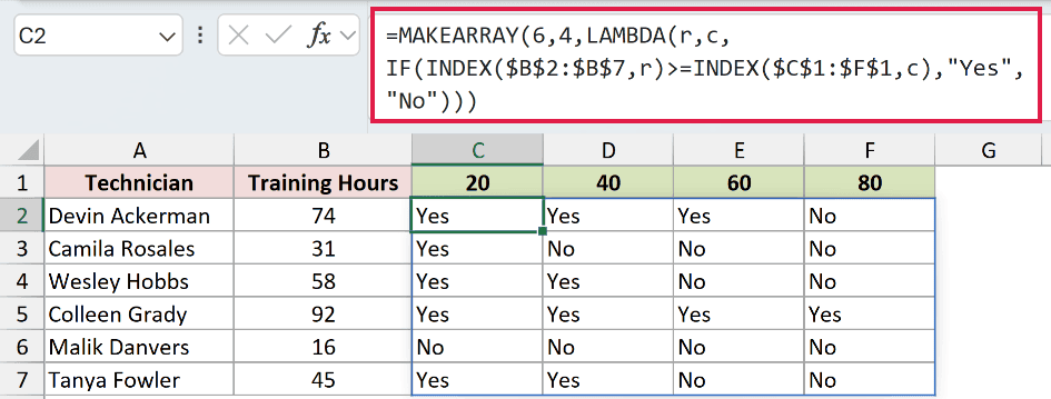
The first INDEX retrieves the technician’s hours. The second retrieves the threshold for the current result column.

IF returns Yes when the hours meet or exceed that threshold. Colleen Grady clears all four levels, while Malik Danvers clears none.

The same result can be returned more directly with =IF(B2:B7>=C1:F1,"Yes","No"). MAKEARRAY gives you room to add a more involved test for each position.

Example 5: Build a Compound Growth Grid

Next, we’ll use the row position as a value instead of only as a lookup position.

Below is the dataset. Column A shows years 1 through 10 as axis labels, while B1:E1 contains annual rates from 3% through 6%.

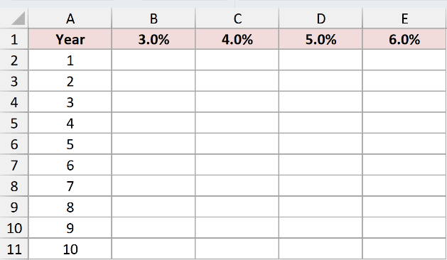
We want to project a $25,000 opening deposit for every year and rate combination. That deposit is hard-coded inside the formula.

Here is the formula:

=MAKEARRAY(10,4,LAMBDA(r,c,25000*(1+INDEX($B$1:$E$1,c))^r))

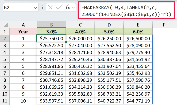
INDEX uses c to retrieve the rate. The row position r becomes the exponent, so the first spilled row calculates year 1.

Column A is only an axis label. The formula does not read A2:A11.

At 3%, the deposit grows to $27,318.18 after three years. At 6%, it reaches $44,771.19 after ten years.

This grid can replace a two-variable What-If Data Table. Unlike that dialog-based tool, the calculation lives in one regular worksheet formula.

Example 6: Calculate Share of Channel Sales

Finally, let’s calculate each product line’s share of its own sales channel.

Below is the dataset. Rows contain five product lines, while columns B:E contain Retail, Online, Wholesale, and Export sales.

We want each value in G:J to show a product line’s percentage of the corresponding channel total.

Here is the formula:

=MAKEARRAY(5,4,LAMBDA(r,c,INDEX($B$2:$E$6,r,c)/SUM(CHOOSECOLS($B$2:$E$6,c))))

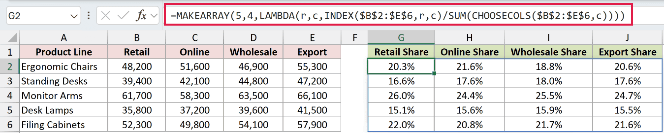
INDEX retrieves the source value at the current row and column. CHOOSECOLS retrieves that whole source column, and SUM calculates its total.

For example, Ergonomic Chairs account for 20.3% of Retail sales and 21.6% of Online sales.

Each result column adds up to 100%, give or take a tenth once the displayed figures are rounded.

MAP passes the lambda a value. MAKEARRAY passes it a position.

That position is what lets this formula choose the correct channel total for every cell.

Tips & Common Mistakes

• Use SEQUENCE for a plain list, row, date run, or evenly stepped grid. MAKEARRAY is for results that depend on position or worksheet lookups.
• Keep the target block empty. Any existing value in the spill area causes a #SPILL! error.
• Edit the formula in the anchor cell. Other cells in the spilled block show the same formula greyed out in the formula bar.
• Use exactly two LAMBDA parameters in row-then-column order. A different parameter count returns #VALUE!.
• Keep rows and cols above zero and numeric. Zero, negative, or non-numeric sizes return #VALUE!.
• A non-integer row or column count returns #VALUE!. Wrap a calculated size in INT or ROUND before passing it to MAKEARRAY.
• Return one value from the LAMBDA for each position. Returning another array from each cell creates a #CALC! error.
• Use RANDARRAY for a plain random grid. MAKEARRAY with RANDBETWEEN also recalculates whenever Excel recalculates.
• Watch performance with large arrays. A 9 by 9 block runs the LAMBDA 81 times, and an expensive calculation runs once for every result cell.

I used six examples to show how MAKEARRAY builds multiplication, commission, code, comparison, growth, and percentage grids.

I also covered how row and column positions pull worksheet values into the LAMBDA and produce a complete spilled array.

List of All Excel Functions

Related Excel Functions / Articles:

• BYROW Function in Excel
• CHOOSE Function in Excel
• MMULT Function in Excel

Other Excel articles you may also like:

• TAKE in Excel