
Excel’s EXPON.DIST function returns the exponential distribution for a specified value and rate. It commonly models waiting times between independent events that occur at a constant average rate.
Set the cumulative argument to TRUE for a probability up to a limit. Set it to FALSE for probability density, which has a different interpretation.
In this article, I’ll show you how to calculate probabilities within, beyond, and between time limits, compare density with cumulative results, and test different average intervals.
EXPON.DIST Function Syntax in Excel
The EXPON.DIST function uses the following syntax:
=EXPON.DIST(x,lambda,cumulative)
xis the value at which you want to evaluate the distribution. It must be zero or greater.lambdais the positive rate parameter. It must use the reciprocal of the same time unit asx.cumulativecontrols the returned form. TRUE returns cumulative probability, while FALSE returns probability density.
When to Use EXPON.DIST Function
- Find the probability that the next arrival occurs within a time limit.
- Calculate the chance that a wait exceeds a threshold.
- Measure the probability that an event occurs within a specified window.
- Compare arrival-time probabilities for processes with different average intervals.
- Model time between independent events when the average event rate stays constant.
Example 1: Probability Within Several Time Limits
Let’s start with a support-ticket queue.
Below is the dataset with six time limits and an average interval of 8 minutes between ticket arrivals.
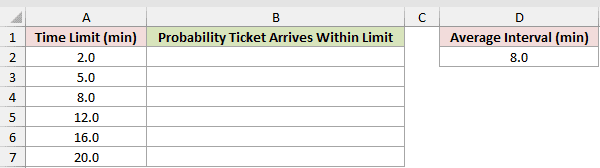
We want to calculate the probability that the next ticket arrives within each listed time limit.
Enter this formula in cell B2:
=EXPON.DIST(A2:A7,1/$D$2,TRUE)
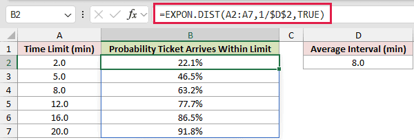
The average interval is 8 minutes, so 1/$D$2 converts it to a rate of 0.125 tickets per minute. The dollar signs keep D2 fixed.
The TRUE argument returns cumulative probabilities. There is a 22.1% chance of a ticket arriving within 2 minutes and a 63.2% chance within 8 minutes.
At 20 minutes, the probability reaches 91.8%. That leaves an 8.2% chance that the next ticket takes longer than 20 minutes.
In Excel 2021, Excel 2024, and Microsoft 365, this array formula spills six results from one cell.
Pro Tip: Keep the units consistent. Because x is measured in minutes here, lambda must be a rate per minute.
Example 2: Probability a Wait Exceeds a Limit
Now let’s calculate a greater-than probability.
Below is the dataset for equipment-support requests that arrive every 0.5 hours on average, with a wait threshold of 1 hour.
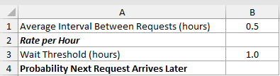
We first want to convert the average interval into the hourly rate required by EXPON.DIST.
Enter this rate formula in cell B2:
=1/B1
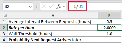
The result is 2.0000 requests per hour. This rate uses the same time unit as the 1-hour threshold in cell B3.
We now want to calculate the probability that the next request arrives later than the 1-hour threshold.
Enter this probability formula in cell B4:
=1-EXPON.DIST(B3,B2,TRUE)
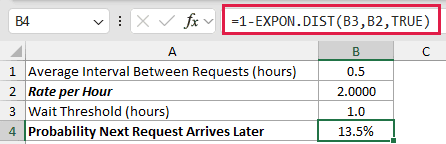
EXPON.DIST with TRUE returns the probability of an arrival within 1 hour. Subtracting that value from 1 returns the remaining tail probability.
The result is 13.5%. Under this model, about 14 out of 100 waits would exceed 1 hour over many observations.
Pro Tip: FALSE returns probability density. It does not return the probability that the wait exceeds x, so use 1 minus the cumulative result.
Example 3: Probability Between Two Times
Here’s a delivery-window example.
Below is the dataset for replacement deliveries averaging 10 minutes apart, with a target window starting after 5 minutes and ending by 12 minutes.
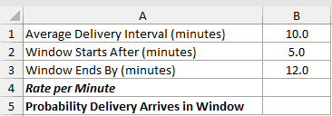
We first want to calculate the delivery rate per minute from the 10-minute average interval.
Enter this rate formula in cell B4:
=1/B1
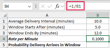
The formula returns 0.1000 deliveries per minute. That rate becomes the lambda argument in the next calculation.
We want to find the probability that the next delivery arrives after 5 minutes but no later than 12 minutes.
Enter this interval formula in cell B5:
=EXPON.DIST(B3,B4,TRUE)-EXPON.DIST(B2,B4,TRUE)
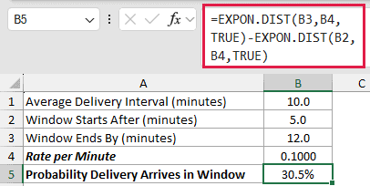
The first EXPON.DIST call calculates cumulative probability through 12 minutes. The second calculates cumulative probability through 5 minutes.
Subtracting the earlier cumulative result isolates the probability inside the window. The result is 30.5%.
This subtraction pattern works for any two valid boundaries when the time-between-events model and constant-rate assumption fit the process.
Example 4: Cumulative Probability Versus Density
This example separates two results that are easy to confuse.
Below is the dataset for website signups that arrive every 6 minutes on average, evaluated at times from 0 through 10 minutes.
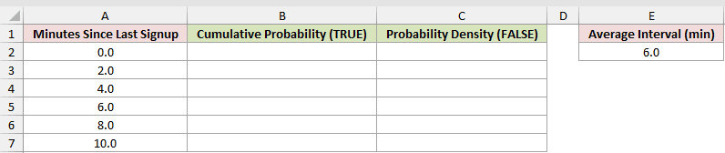
We first want the probability that the next signup has arrived by each listed time.
Enter this cumulative formula in cell B2:
=EXPON.DIST(A2:A7,1/$E$2,TRUE)
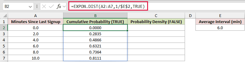
The cumulative values rise as time passes. At 6 minutes, 0.6321 means there is a 63.21% chance that the next signup has already occurred.
We also want the probability density at each listed time.
Enter this density formula in cell C2:
=EXPON.DIST(A2:A7,1/$E$2,FALSE)
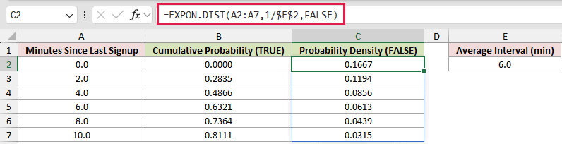
The density starts at 0.1667 and falls over time. At 6 minutes, it is 0.0613 per minute.
Density is the curve’s height at a point, not the probability of an arrival at that exact time. Use cumulative differences to calculate probability over an interval.
Pro Tip: A continuous distribution assigns zero probability to one exact time. The FALSE result becomes useful when you study the curve or calculate probability across a range.
Example 5: Compare Different Average Intervals
Let’s finish by comparing several service queues.
Below is the dataset with four mean request intervals and a common wait target of 5 minutes.

We want to compare the probability that the next request arrives within 5 minutes for each average interval.
Enter this formula in cell B2:
=EXPON.DIST($D$2,1/A2:A5,TRUE)
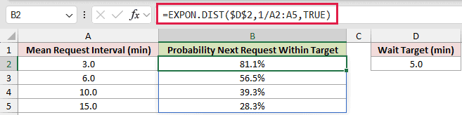
The formula keeps the 5-minute target fixed and converts every mean interval in A2:A5 to its corresponding rate.
A 3-minute mean interval produces an 81.1% probability. The probability falls to 28.3% when the mean interval increases to 15 minutes.
Shorter average intervals correspond to higher arrival rates, so a request is more likely to arrive within the same 5-minute target.
Pro Tip: Use this comparison only when each queue reasonably follows a constant-rate exponential model. Real arrival patterns may vary by hour, weekday, or workload.
Tips & Common Mistakes
- Convert a mean interval to a rate with
1/mean. Passing the mean itself as lambda changes the model and produces the wrong probabilities. - Keep
xand lambda in matching units. Minutes require a per-minute rate, while hours require a per-hour rate. - Use TRUE for cumulative probability through
x. Use1-EXPON.DIST(x,lambda,TRUE)for a probability beyondx. - Use FALSE for probability density, not for the probability that an event occurs at one exact time.
- A negative
xor a lambda of zero or less returns#NUM!. Nonnumericxor lambda returns#VALUE!. - Spilled formulas need empty destination cells. A blocked output range returns a
#SPILL!error in dynamic-array versions of Excel. - Use EXPON.DIST in new work. The older EXPONDIST function remains available for compatibility, but Microsoft recommends the newer name.
- Confirm that a constant average event rate is a reasonable assumption. If failure risk changes over time, another distribution such as WEIBULL.DIST may fit better.
EXPON.DIST can calculate probabilities within a deadline, beyond a threshold, or between two times. It also lets you compare how different average intervals affect the same target.
I hope you found this article helpful.
Other Excel articles you may also like:
