
The LOGNORM.DIST function in Excel returns a cumulative probability or probability density for a lognormal distribution.
This model describes positive values with a long right tail, such as repair times where most jobs finish fairly quickly but some take much longer.
LOGNORM.DIST needs the mean and standard deviation of the natural logarithms, not the original measurements.
I’ll show you how to calculate deadline probabilities, estimate the log parameters from data, and convert a reported average and standard deviation without getting a misleading answer.
LOGNORM.DIST Function Syntax in Excel
LOGNORM.DIST takes four required arguments:
=LOGNORM.DIST(x,mean,standard_dev,cumulative)
- x: The positive value you want to evaluate, in the original units, such as hours or dollars.
- mean: The mean of the natural logarithms of the values. This can be negative.
- standard_dev: The standard deviation of those natural logarithms. It must be greater than zero.
- cumulative: Use
TRUEfor the probability of a value at or belowx. UseFALSEfor density, the height of the distribution curve.
You must supply cumulative. Leaving it out causes Excel to reject the formula when you enter it.
LOGNORM.DIST is available in Excel 2010 and later.
When to Use LOGNORM.DIST Function
- Estimate the share of files at or below a size limit under a lognormal model.
- Calculate the chance that a repair exceeds a deadline or falls within a time window.
- Estimate a claim probability after calculating log parameters from recorded claim amounts.
- Compare density and cumulative probability across session lengths.
- Use a reported average and standard deviation after converting them to log parameters.
Example 1: Calculate Probabilities Across File Sizes
Let’s start with file sizes on a shared drive.
Below is the dataset. Columns A:B list files and sizes, E2:F2 hold log parameters, and column C has a header and empty cells for probabilities.
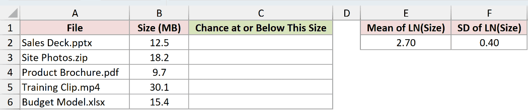
We want the modeled probability of a file being at or below each listed size.
Enter this formula in C2:
=LOGNORM.DIST(B2:B6,E2,F2,TRUE)
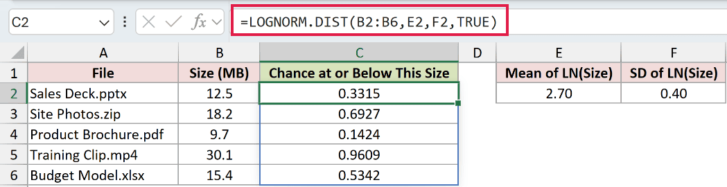
The formula spills into C2:C6. It evaluates every size in B2:B6 using the same log mean of 2.70 and log standard deviation of 0.40.
For Sales Deck.pptx at 12.5 MB, C2 returns 0.3315. Training Clip.mp4 at 30.1 MB returns 0.9609 in C5.
These probabilities describe the supplied model rather than the share of files below each size in this short list.
NORM.DIST calculates normal-distribution probabilities; here, the natural logarithms of lognormal file sizes follow a normal distribution described by the parameters in E2:F2.
Evaluating each size’s natural logarithm with those parameters and TRUE therefore returns the same cumulative probabilities as column C.
Range formulas spill in Excel 2021, Excel 2024, and Microsoft 365. In Excel 2019 and earlier, use a per-row version copied down, keeping the parameter references fixed.
Example 2: Find Above and Between Probabilities
A repair deadline calls for a different part of the same distribution.
Below is the dataset. B1:B5 hold the log parameters, deadline, and time limits; the labeled cells B6:B8 are reserved for the probabilities.
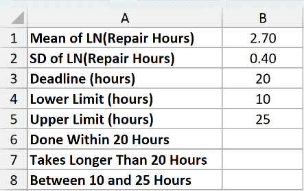
We want the chances of finishing within 20 hours, taking longer, and finishing between 10 and 25 hours.
First, enter the cumulative formula in B6:
=LOGNORM.DIST(B3,B1,B2,TRUE)
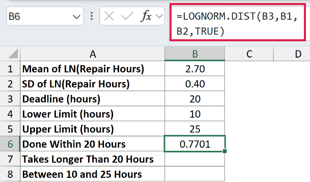
B6 returns 0.7701, the probability of finishing at or before the deadline in B3.
For the right-tail probability of taking longer, enter this in B7:
=1-LOGNORM.DIST(B3,B1,B2,TRUE)
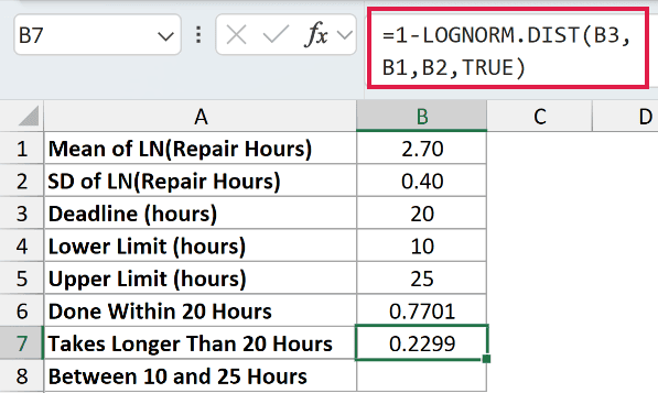
B7 returns 0.2299. Subtracting the cumulative probability from one leaves the probability above the deadline.
For the probability between the limits, enter this in B8:
=LOGNORM.DIST(B5,B1,B2,TRUE)-LOGNORM.DIST(B4,B1,B2,TRUE)
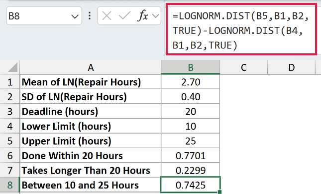
B8 returns 0.7425. The formula takes the cumulative probability at the upper limit and removes everything below the lower limit.
Both calls use TRUE. Subtracting density values wouldn’t calculate the probability of landing within this time window.
Example 3: Get Log Parameters From Claim Data
When you have individual observations, calculate their natural logarithms before estimating the parameters.
Below is the dataset. A:B lists claim IDs and amounts; D:E contains labeled parameter cells, a typed threshold, and space for the exceedance probability.
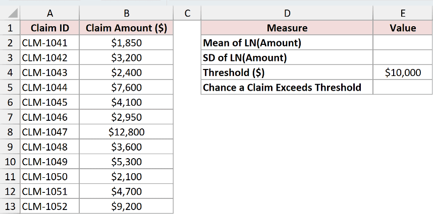
We want to fit the log parameters from the claim amounts and estimate the chance of a claim exceeding $10,000.
Calculate the mean of the natural logarithms in E2:
=AVERAGE(LN(B2:B13))
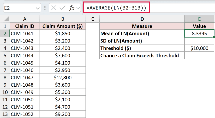
E2 displays 8.3395. LN transforms each amount, and AVERAGE reduces those transformed values to a single mean.
The formulas in E2 and E3 work normally in Excel 2021, Excel 2024, and Microsoft 365. In Excel 2019 and earlier, confirm each with Ctrl+Shift+Enter.
Calculate their sample standard deviation in E3:
=STDEV.S(LN(B2:B13))
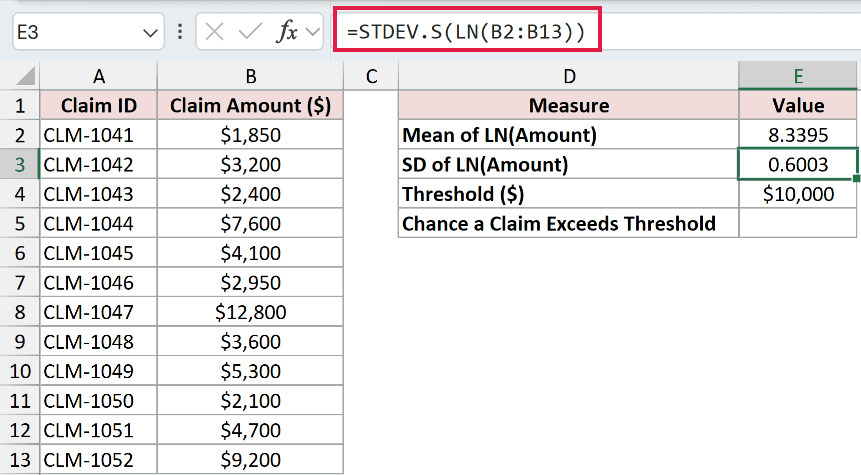
E3 displays 0.6003. This measures the spread of the natural logarithms, rather than the spread of the dollar amounts.
Now calculate the probability above the typed threshold in E5:
=1-LOGNORM.DIST(E4,E2,E3,TRUE)
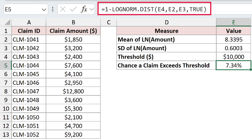
E5 returns 7.34%. That’s the estimated chance of a claim exceeding $10,000 under the fitted lognormal model.
The threshold stays in dollars. Only the data used to estimate the mean and standard deviation goes through LN.
Pro Tip: Reference E2 and E3 in the final formula instead of typing their displayed values. The cells retain more precision than their number formats show.
Example 4: Compare Density and Cumulative Probability
The TRUE/FALSE switch changes what the result means, so let’s put both outputs beside the same session lengths.
Below is the dataset. Column A lists session lengths, E2:F2 contain log parameters, and columns B:C have headers and empty cells for density and cumulative probability.
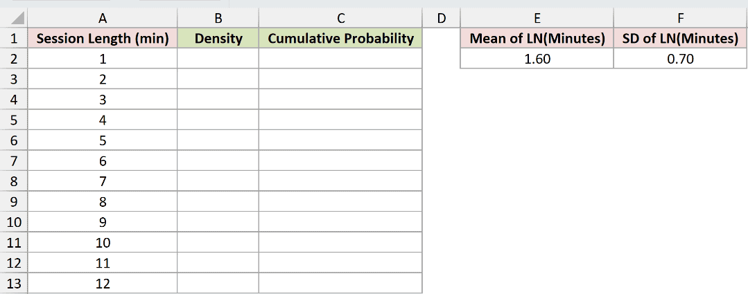
We want to compare the curve height at each session length with the probability of a session ending by that time.
Enter the density formula in B2:
=LOGNORM.DIST(A2:A13,E2,F2,FALSE)
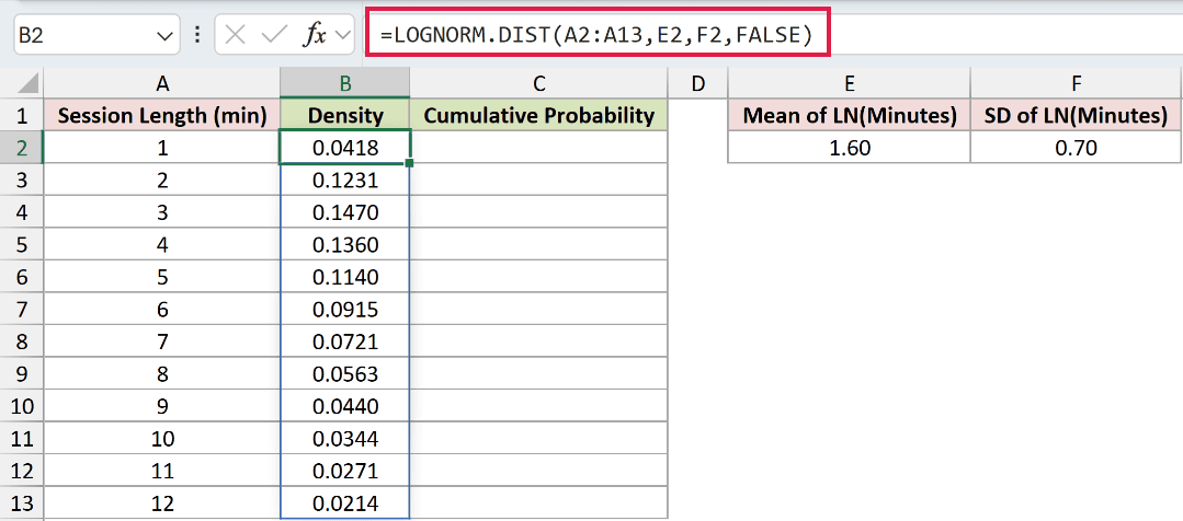
The formula spills into B2:B13. Among the listed session lengths, density is highest at 3 minutes, where B4 displays 0.1470.
That value is a curve height. It isn’t the probability of a session lasting exactly 3 minutes, and you shouldn’t read it as a percentage.
Next, enter the cumulative formula in C2:
=LOGNORM.DIST(A2:A13,E2,F2,TRUE)
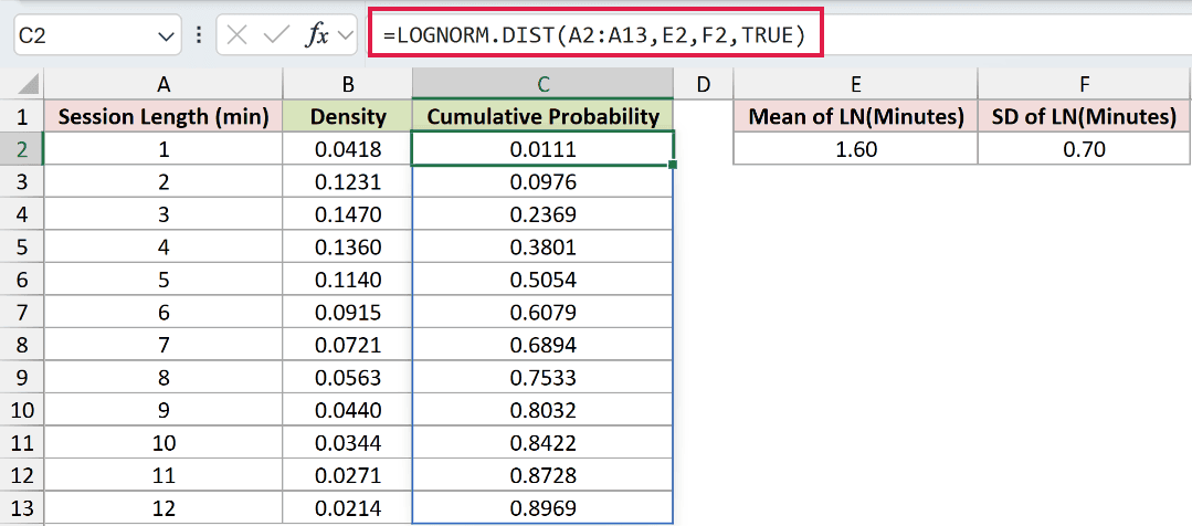
This formula spills into C2:C13. At 3 minutes, C4 returns 0.2369, the probability of a session lasting at most that long.
The cumulative result increases from 0.3801 at 4 minutes to 0.5054 at 5 minutes. The median therefore falls between those session lengths.
Density rises and then falls, while cumulative probability keeps increasing. Use density to inspect the curve’s shape and cumulative values to answer probability questions.
Example 5: Convert a Reported Average and SD
A report may give you the average order value and standard deviation without listing the individual orders.
Below is the dataset. B1:B3 hold the reported average, standard deviation, and order limit; labeled cells below hold converted parameters, the probability, and a deliberate wrong calculation.
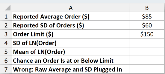
We want the chance of an order being at or below $150, using a reported average of $85 and standard deviation of $60.
First, convert the reported standard deviation to the log standard deviation in B4:
=SQRT(LN(1+(B2/B1)^2))
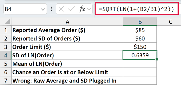
B4 returns 0.6359. Assuming a lognormal distribution, the expression inside SQRT calculates the log variance from the reported average and standard deviation.
SQRT takes the square root of that variance to get the log standard deviation that LOGNORM.DIST needs.
Then calculate the log mean in B5:
=LN(B1)-B4^2/2
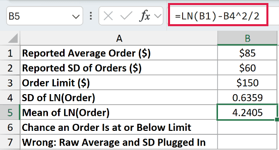
B5 returns 4.2405. The correction after LN accounts for the distribution’s spread. Taking the logarithm of the raw average alone isn’t enough.
Use the converted parameters to calculate the probability in B6:
=LOGNORM.DIST(B3,B5,B4,TRUE)
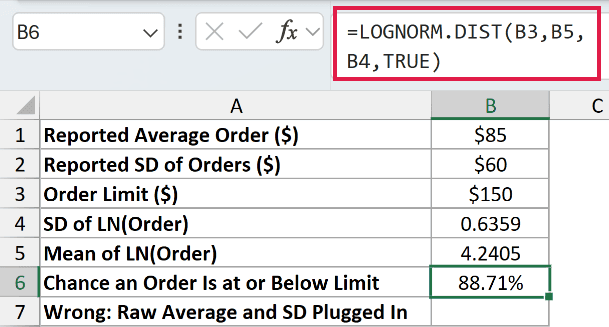
B6 returns 88.71%, the modeled probability of an order being at or below the limit.
For the deliberate mistake in B7, this formula plugs in the raw average and standard deviation. It is what not to do:
=LOGNORM.DIST(B3,B1,B2,TRUE)
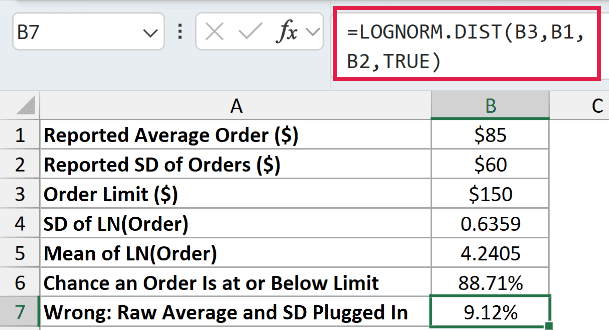
The wrong calculation in B7 returns 9.12%. Excel accepts the numbers, but it interprets them as log parameters and evaluates a different distribution.
Check what your source report means by average and standard deviation before choosing the input cells.
Tips & Common Mistakes
- Use positive values. LOGNORM.DIST returns
#NUM!whenxorstandard_devis zero or negative. A negativemeanis allowed because it describes logarithms. - Choose TRUE or FALSE deliberately.
TRUEreturns cumulative probability;FALSEreturns density. Text such as"yes"in the cumulative argument returns#VALUE!. - Keep the threshold in its original units. Hours stay hours and dollars stay dollars. The mean and standard deviation describe the natural logarithms of those values.
- Don’t confuse the mean with the median. Exponentiating the log mean gives the median. The arithmetic mean of a lognormal distribution is higher.
- Use LOGNORM.INV for the reverse question. It returns the value associated with a target cumulative probability, such as a repair-time cutoff.
- Recognize the older name. LOGNORMDIST remains available for compatibility and calculates cumulative probabilities only.
Related Excel Functions / Articles:
