
Excel’s F.DIST function returns the cumulative probability or probability density for an F distribution, depending on its final argument.
The cumulative result tells you how much of the distribution lies at or below an F statistic.
I’ll show you how to compare density with cumulative probability, calculate a left-tail result from sample data, and find probabilities between two ratio limits.
F.DIST Function Syntax in Excel
The F.DIST function has four required arguments:
=F.DIST(x,deg_freedom1,deg_freedom2,cumulative)
- x: The nonnegative F value where you want to evaluate the distribution.
- deg_freedom1: The numerator degrees of freedom. For a sample variance ratio, this is the numerator sample size minus one.
- deg_freedom2: The denominator degrees of freedom. For a sample variance ratio, this is the denominator sample size minus one.
- cumulative: Use TRUE for the probability at or below x, or FALSE for the density, which is the curve’s height at x.
When to Use F.DIST Function
- Find left-tail probabilities for F statistics you already have.
- Build a table of density and cumulative values for an F distribution.
- Evaluate a smaller sample variance against a comparison sample.
- Calculate a two-tailed p-value from sample sizes and standard deviations.
- Find the probability that a variance ratio falls between two limits.
Example 1: Calculate Left-Tail F Distribution Probabilities
Let’s start with F statistics that have already been calculated for several oven pairs.
Below is the dataset with oven pairs, F statistics, both degrees of freedom, and empty cells under Probability to the Left.
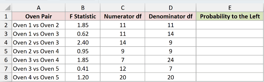
We want to calculate the probability at or below each F statistic, using that row’s degrees of freedom.
Here is the formula:
=F.DIST(B2:B8,C2:C8,D2:D8,TRUE)
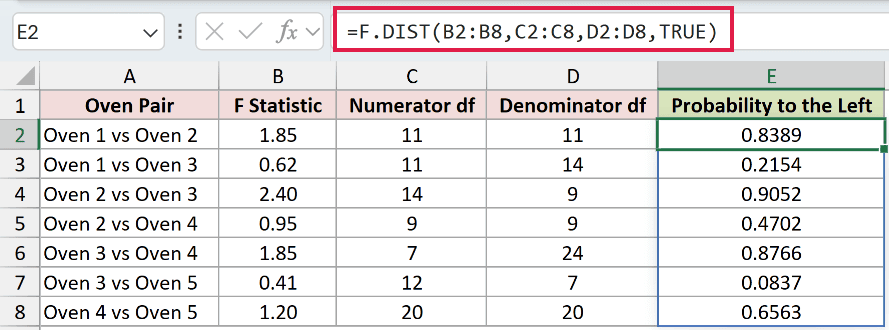
Enter it in E2. In Excel 2021, Excel 2024, and Microsoft 365, the seven results spill into E2:E8 automatically.
How this formula works:
- B2:B8 supplies the F statistics.
- C2:C8 and D2:D8 supply the matching numerator and denominator degrees of freedom for each row.
- TRUE requests cumulative probability, so each result represents the area to the left of that row’s F statistic.
For Oven 1 vs Oven 2, an F statistic of 1.85 with 11 and 11 degrees of freedom returns 0.8389, or about 83.89%.
Oven 3 vs Oven 4 also has an F statistic of 1.85. Its degrees of freedom are 7 and 24, so its probability is different: 0.8766.
Pro Tip: In Excel 2019 and earlier, use single-row references for the F statistic and both degrees of freedom, then fill down. The range-based formula above requires dynamic arrays.
Example 2: Compare F.DIST TRUE and FALSE
The same F values can give you a density curve or a cumulative probability curve.
Below is the dataset with F values from 0 to 4, empty Density and Cumulative Probability columns, and degrees of freedom in E2:F2.
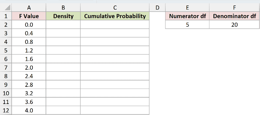
We want to calculate the density at each F value, using 5 numerator and 20 denominator degrees of freedom.
Here is the formula:
=F.DIST(A2:A12,E2,F2,FALSE)
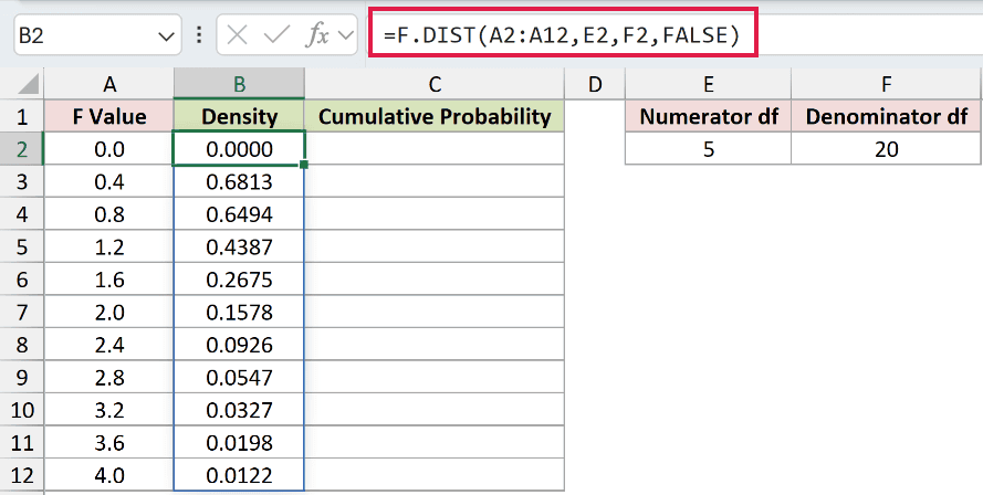
Enter the formula in B2. It spills density values into B2:B12, reusing the degrees of freedom in E2 and F2 for every row.
Next, enter this formula in C2 to calculate cumulative probabilities for the same F values:
=F.DIST(A2:A12,E2,F2,TRUE)
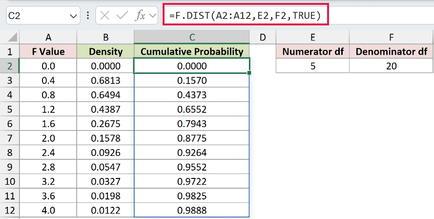
At an F value of 0.4, the density is 0.6813, while the cumulative probability is 0.1570.
The first number describes the curve’s height. The second means about 15.70% of the distribution lies at or below 0.4.
At an F value of 4, density has fallen to 0.0122, while cumulative probability has risen to 0.9888.
You now have a table for plotting either curve. Changing E2 or F2 recalculates both columns for a different F distribution.
Pro Tip: A density is not the probability of getting exactly that F value. Keep the Density column numeric, and use the cumulative column when you need a probability.
Example 3: Compare Grinder Variability From Sample Data
This time, we’ll calculate the F statistic from individual measurements.
Below is the dataset with 12 yields per grinder, calculated variances and degrees of freedom, an F statistic, and an empty labeled cell for left-tail probability.
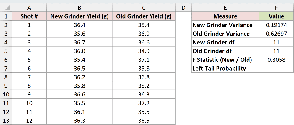
We want to evaluate whether the new grinder’s smaller sample variance produces an unusually low ratio compared with the old grinder.
Here is the formula:
=F.DIST(F6,F4,F5,TRUE)
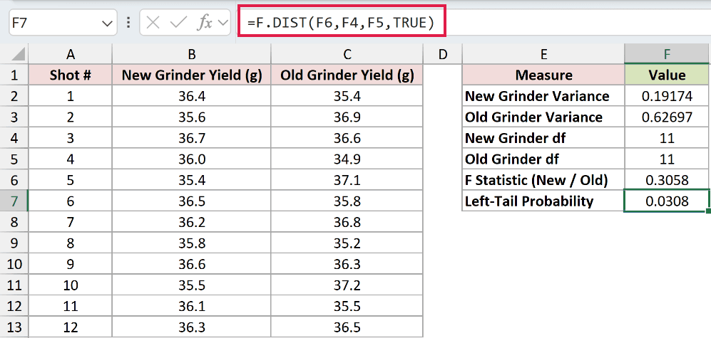
Enter it in F7 to calculate the left-tail probability.
How the card is built:
- F2 uses
=VAR.S(B2:B13)to calculate the new grinder’s sample variance, displayed as 0.19174. - F3 uses
=VAR.S(C2:C13)for the old grinder’s sample variance, displayed as 0.62697. - F4 uses
=COUNT(B2:B13)-1. The new grinder has 12 numeric measurements, giving 11 degrees of freedom. - F5 uses
=COUNT(C2:C13)-1. The old grinder also has 12 measurements, giving 11 degrees of freedom. - F6 uses
=F2/F3, returning 0.3058. The new grinder’s sample variance is about 30.58% of the old grinder’s.
How this formula works:
- F6 supplies the new-to-old variance ratio, approximately 0.3058.
- F4 supplies the numerator degrees of freedom, 11.
- F5 supplies the denominator degrees of freedom, also 11.
- TRUE returns the probability at or below that ratio under the F distribution.
The result is 0.0308, or about 3.08%. A ratio this low lies near the left edge of the reference distribution.
Pro Tip: Interpreting this as a one-sided variance test requires independent samples from normal populations and a lower-variance hypothesis chosen before examining the results. Keep new variance on top and its degrees of freedom first. Swapping the samples changes the tail you’re reading.
Example 4: Find a Two-Tailed p-Value From Summaries
Sometimes you have sample sizes and standard deviations without the individual observations.
Below is the dataset with student counts and standard deviations for two sections, a calculated F statistic, and empty labeled cells for the probabilities.
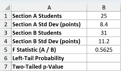
We want to calculate a two-tailed p-value for a difference in score variability between the two sections.
Here is the formula:
=F.DIST(B5,B1-1,B3-1,TRUE)
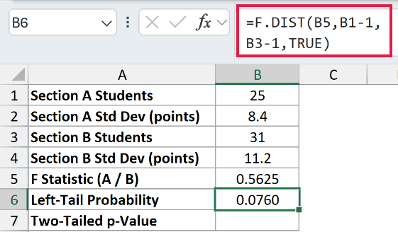
Enter it in B6. Cell B5 already uses =B2^2/B4^2 to square the standard deviations, 8.4 and 11.2, then divide the variances. The ratio is 0.5625.
The sample sizes are 25 and 31, giving 24 numerator and 30 denominator degrees of freedom. F.DIST returns 0.0760.
To account for a difference in either direction, enter this formula in B7:
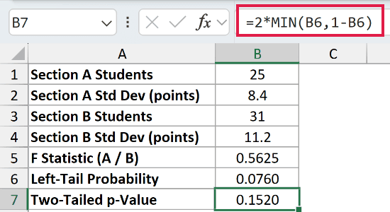
=2*MIN(B6,1-B6)
How this formula works:
- B6 contains the left-tail probability, approximately 0.0760.
- 1-B6 calculates the remaining probability in the right tail.
- MIN selects the smaller tail probability.
- Multiplying by 2 returns the two-tailed p-value, displayed as 0.1520.
At a 5% significance level, this result doesn’t provide enough evidence to reject equal population variances.
Pro Tip: This variance test assumes independent samples from normal populations. With raw observations, F.TEST calculates a two-tailed p-value directly. The summary-based approach here works when you only have sample sizes and sample standard deviations.
Example 5: Calculate Probability Between Two F Values
You can also subtract cumulative probabilities to find the area between two ratio limits.
Below is the dataset with five ratio bands, empty Chance Inside Band cells, and sample counts of 15 readings for each scale.
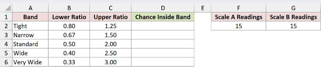
We want the probability that a sample variance ratio falls inside each band under an equal-population-variance model.
Here is the formula:
=F.DIST(C2:C6,F2-1,G2-1,TRUE)-F.DIST(B2:B6,F2-1,G2-1,TRUE)
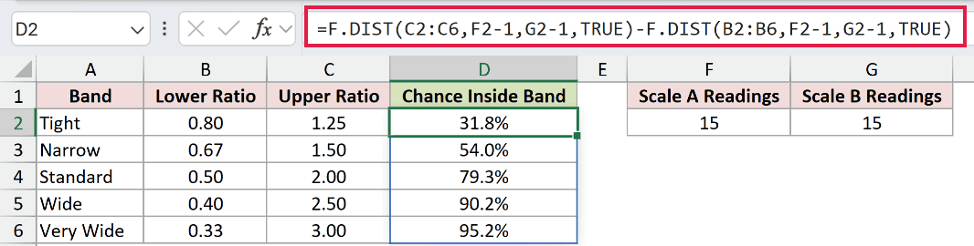
Enter it in D2. The results spill into D2:D6 and display as percentages.
How this formula works:
- F2-1 and G2-1 convert the two sample sizes of 15 into 14 degrees of freedom each.
- The first F.DIST calculates the cumulative probability at each upper ratio in C2:C6.
- The second calculates the cumulative probability at each lower ratio in B2:B6.
- Subtracting the lower cumulative probability from the upper one leaves the probability inside each band.
The Tight band, from 0.80 to 1.25, contains 31.8% of the distribution. The Standard band, from 0.50 to 2.00, contains 79.3%.
Widening the limits to 0.33 and 3.00 increases the probability to 95.2%.
Pro Tip: These are probabilities under an equal-variance model with independent normal samples. They are not probabilities that the scales have equal variances, and a wide band alone does not establish acceptable scale performance.
Tips & Common Mistakes
- Choose the correct mode. TRUE returns cumulative probability. FALSE returns density. Enter the argument explicitly so the intended calculation is clear.
- Check which tail you need. F.DIST with TRUE returns the left tail. F.DIST.RT returns the right tail directly.
- Keep the variance order consistent. The first degrees-of-freedom argument belongs to the numerator sample, and the second belongs to the denominator sample.
- Square standard deviations first. An F statistic for comparing variances uses a ratio of variances, as shown in Example 4.
- Check invalid inputs. Negative x values or degrees of freedom below 1 return #NUM!. Nonnumeric inputs can return #VALUE!.
- Use the intended degrees of freedom. Excel truncates noninteger degrees of freedom rather than rounding them.
- Leave spill destinations empty. Occupied cells can cause #SPILL!. Enter each spilling formula once, in its top-left result cell.
Try changing the ratio limits in Example 5 to see how much the coverage changes.
You can use the same setup to compare bands that fit your own measurements.
Other Excel articles you may also like:
