
The F.INV function in Excel returns the F value for a given cumulative probability and degrees of freedom. The probability measures the area to the left.
A small probability returns a lower cutoff, which helps you test whether a new process is less variable than an existing one.
We’ll start with lower cutoffs, then use them to compare machine variability. The final example builds a confidence interval for a variance ratio.
F.INV Function Syntax in Excel
F.INV takes these required arguments:
=F.INV(probability,deg_freedom1,deg_freedom2)
- probability is the cumulative probability to the left of the F value. Use a number from 0 up to, but not including, 1.
- deg_freedom1 is the numerator’s degrees of freedom. For a sample variance, use the sample size minus 1.
- deg_freedom2 is the denominator’s degrees of freedom, calculated from the sample used in the denominator.
Keep the degrees of freedom in the same order as the variances in your ratio. F.INV is available in Excel 2010 and later.
When to Use F.INV Function
- Find lower F cutoffs for different sample sizes.
- Turn cumulative probabilities into F values for a percentile table.
- Test whether a replacement machine produces less variable measurements.
- Calculate both limits for a comparison of instrument precision.
- Build a confidence interval for the ratio of population variances.
Example 1: Find Lower Cutoffs for Field Trials
Let’s start with fertilizer trials that use different numbers of plots.
Below is the dataset. Columns B and C hold plot counts for each blend, F2 holds the probability, and column D will show the lower cutoffs.
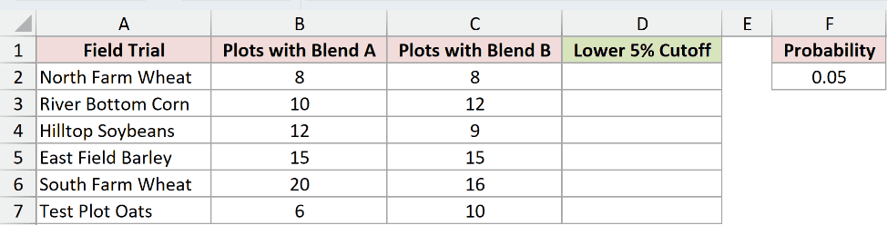
We want the lower 5% cutoff for every trial, using each blend’s plot count to calculate its degrees of freedom.
Enter this formula in D2:
=F.INV(F2,B2:B7-1,C2:C7-1)
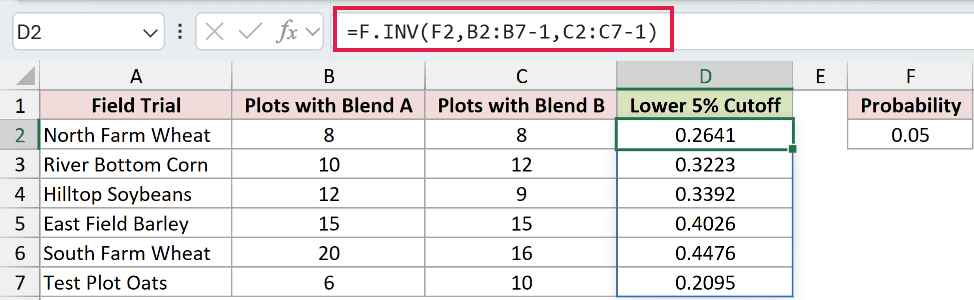
The formula spills into D2:D7. Subtracting 1 from each plot count supplies the degrees of freedom, while F2 supplies the same probability for every row.
North Farm Wheat returns 0.2641, and East Field Barley returns 0.4026. The cutoff depends on the sample sizes even though the probability stays unchanged.
These are lower-tail cutoffs for a Blend A variance divided by a Blend B variance.
This range formula spills in Excel 2021, Excel 2024, and Microsoft 365. In Excel 2019 and earlier, use individual row references and fill down, keeping the probability reference fixed.
Example 2: Build an F Percentile Table
Now let’s see what happens when the probability changes and the degrees of freedom stay fixed.
Below is the dataset. Column A holds cumulative probabilities, E2:F2 holds the degrees of freedom, and columns B:C are reserved for F values and a round-trip check.
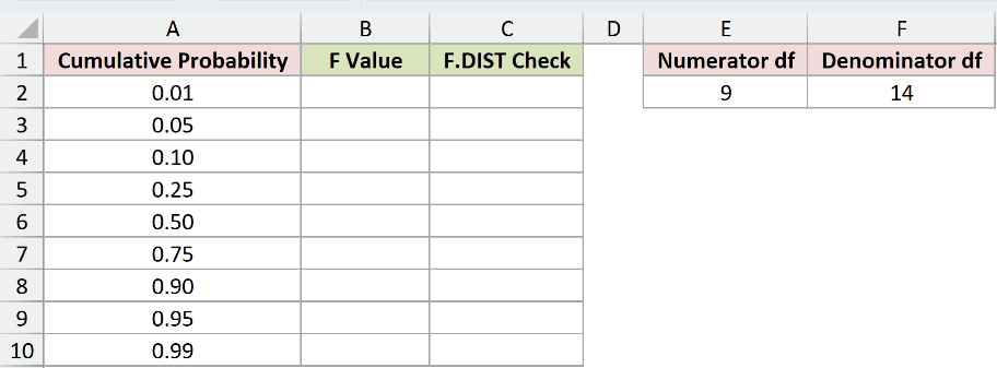
We want the F value at each probability, then a check that F.DIST recovers the original probability.
Enter the F.INV formula in B2:
=F.INV(A2:A10,E2,F2)
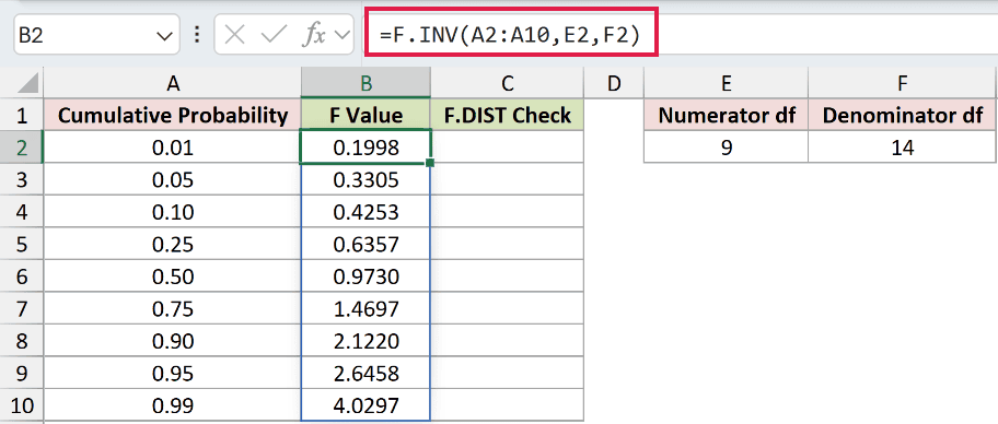
The results spill into B2:B10 using numerator df 9 and denominator df 14.
At probability 0.50, F.INV returns 0.9730. That’s the median of this F distribution, and it falls below 1.
At 0.95, the result is 2.6458; at 0.99, it’s 4.0297. The upper end stretches out because the distribution is skewed.
For the round-trip check in column C, enter this formula in C2:
=F.DIST(B2:B10,E2,F2,TRUE)
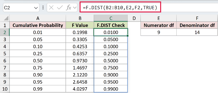
This check spills into C2:C10. The TRUE argument asks F.DIST for cumulative probabilities, reversing the job F.INV performed.
The check displays 0.0100 in C2, 0.5000 in C6, and 0.9900 in C10, matching the corresponding inputs. Column C verifies the F values; it isn’t another cutoff column.
Example 3: Test Whether a Lathe Is Less Variable
A replacement lathe should produce more consistent shaft diameters, so let’s test for reduced variability.
Below is the dataset. Columns B:C contain new and old lathe diameters in millimeters, while the E:F card has labels and result cells for the comparison.
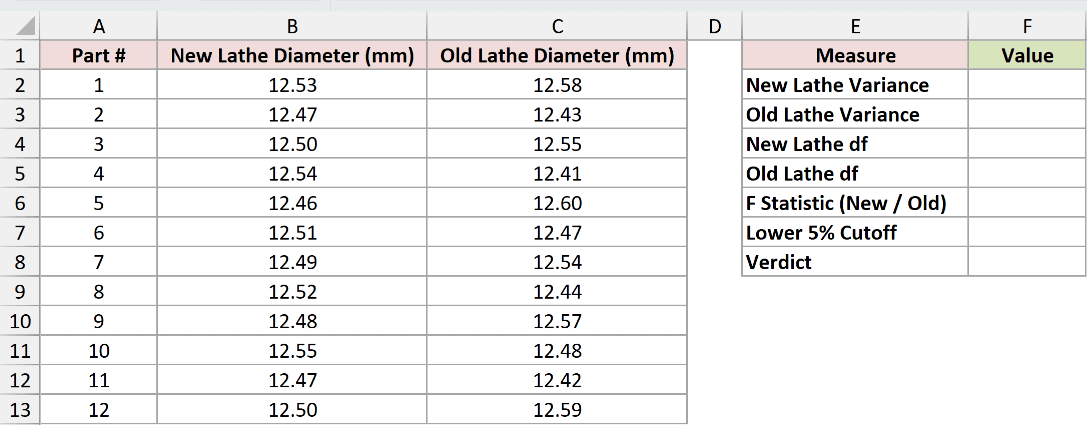
We want to compare the new-to-old variance ratio with a lower cutoff at the 5% significance level.
Calculate the new lathe’s sample variance in F2:
=VAR.S(B2:B13)
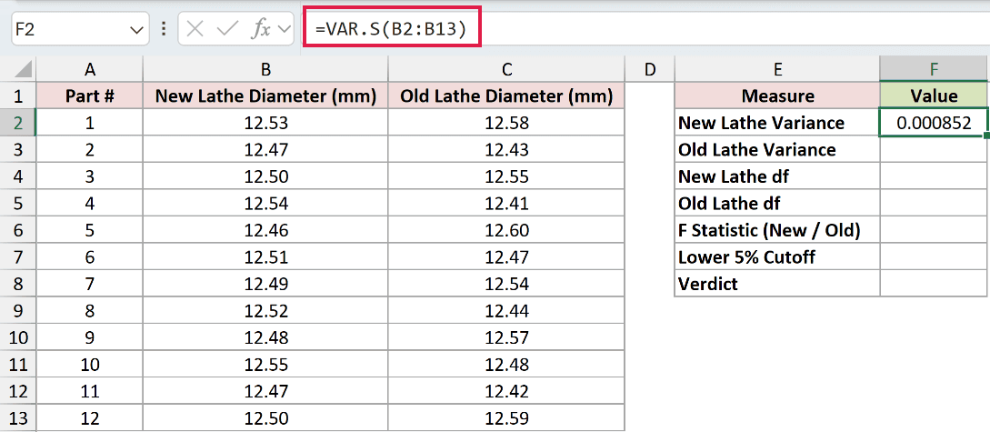
F2 displays 0.000852. Next, calculate the old lathe’s sample variance in F3:
=VAR.S(C2:C13)
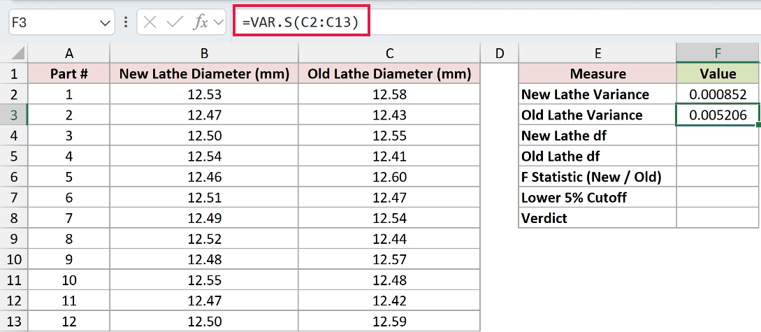
F3 displays 0.005206. Use COUNT minus 1 to calculate the new lathe’s degrees of freedom in F4:
=COUNT(B2:B13)-1
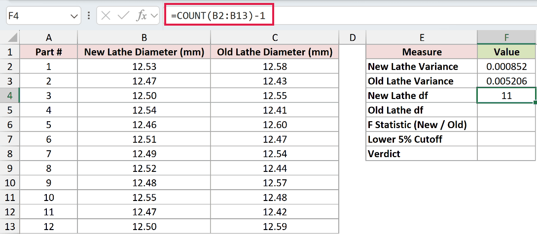
F4 returns 11. Calculate the old lathe’s degrees of freedom in F5:
=COUNT(C2:C13)-1
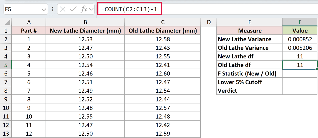
F5 also returns 11. Now divide the new variance by the old variance in F6:
=F2/F3
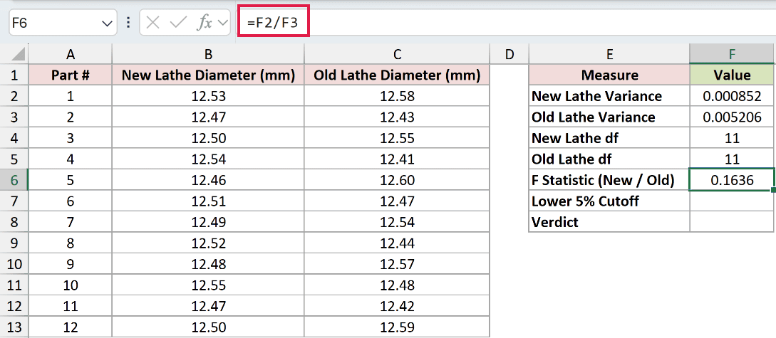
The F statistic is 0.1636. Keep the new variance on top because the question is whether that variance is smaller.
Calculate the lower cutoff in F7:
=F.INV(0.05,F4,F5)
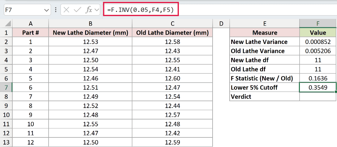
F.INV returns 0.3549. An observed ratio below this cutoff supports reduced variability in the new lathe.
Finally, use IF for the decision formula in F8:
=IF(F6<F7,"New lathe is less variable","No significant difference")
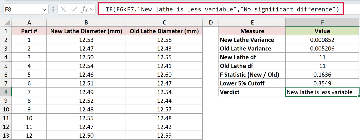
The result is New lathe is less variable, because 0.1636 is below 0.3549. The test compares how widely the diameter measurements vary.
Example 4: Compare Precision in Either Direction
When comparing pH meters, you may want to detect a precision difference in either direction.
Below is the dataset. The card holds each meter’s validation-run count, standard deviation, and significance level, followed by labeled cells for the statistic, limits, and verdict.
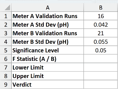
We want lower and upper cutoffs for a two-sided comparison of the meters’ variances.
Calculate the variance ratio in B6:
=B2^2/B4^2
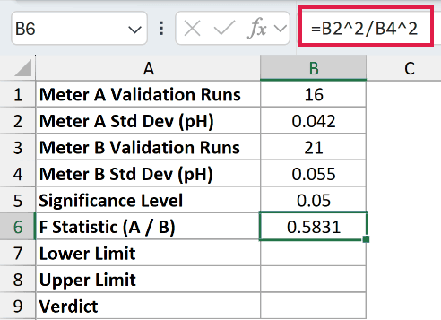
Squaring each standard deviation converts it to a variance. Meter A’s variance divided by Meter B’s variance returns 0.5831.
Calculate the lower limit in B7:
=F.INV(B5/2,B1-1,B3-1)
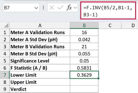
The lower limit is 0.3629. Dividing the significance level between the tails lets the test detect unusually small and unusually large ratios.
Calculate the upper limit in B8:
=F.INV(1-B5/2,B1-1,B3-1)
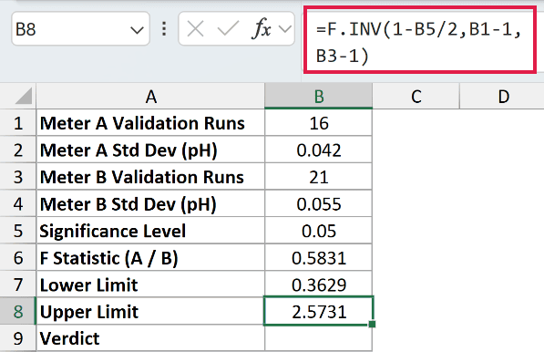
The upper limit is 2.5731. F.INV still uses a left-tail probability here, so the formula subtracts the upper-tail share from 1.
Use AND inside IF to check whether the statistic falls between the limits in B9:
=IF(AND(B6>=B7,B6<=B8),"Same precision","Precision differs")
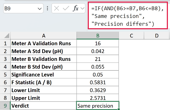
The worksheet returns Same precision because 0.5831 falls between 0.3629 and 2.5731.
Pro Tip: Treat the worksheet’s “Same precision” label as no statistically significant difference at the chosen significance level. It doesn’t prove the population variances are identical.
Example 5: Estimate a Variance Ratio Interval
Let’s finish with a range of plausible variance ratios for corn yields under different irrigation methods.
Below is the dataset. Columns B:C hold drip and center-pivot yields in bushels per acre, while E:F provides labeled cells for variances, their ratio, and interval bounds.
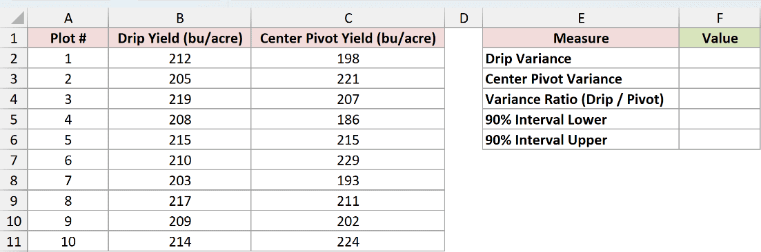
We want a 90% confidence interval for the drip-to-center-pivot population variance ratio.
Calculate the drip yield variance in F2:
=VAR.S(B2:B11)
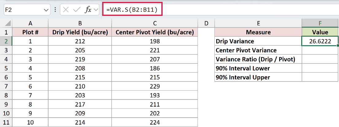
F2 displays 26.6222. Calculate the center-pivot yield variance in F3:
=VAR.S(C2:C11)
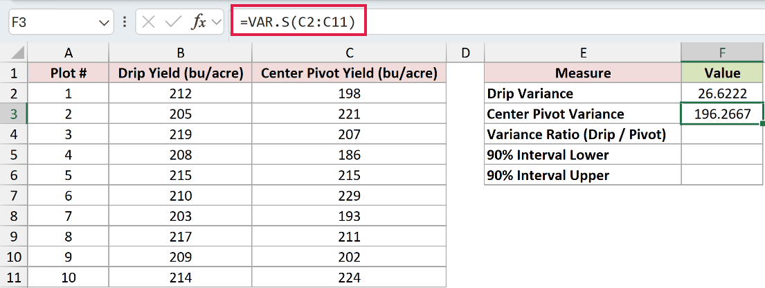
F3 displays 196.2667. Calculate the sample variance ratio in F4:
=F2/F3
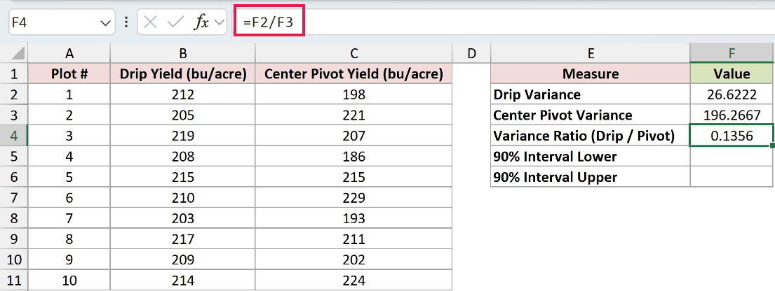
The ratio is 0.1356. Now calculate the lower confidence bound in F5:
=F4/F.INV(0.95,COUNT(B2:B11)-1,COUNT(C2:C11)-1)
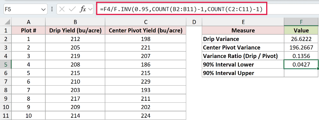
The lower bound is 0.0427. The lower confidence bound divides the observed ratio by the upper F quantile.
Calculate the upper confidence bound in F6:
=F4/F.INV(0.05,COUNT(B2:B11)-1,COUNT(C2:C11)-1)
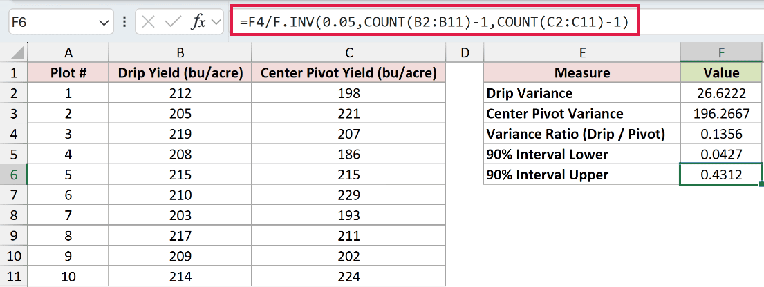
The upper bound is 0.4312. Dividing by the smaller F quantile produces the larger confidence bound.
The 90% confidence interval runs from 0.0427 to 0.4312. It lies entirely below 1, supporting lower yield variability under drip irrigation.
This interval estimates how variable drip yields are relative to center-pivot yields.
Tips & Common Mistakes
- Choose the correct tail. For an ANOVA upper cutoff at a 5% significance level, supply probability 0.95 to F.INV, or use F.INV.RT with 0.05. Supplying 0.05 to F.INV produces a lower cutoff.
- Keep the numerator and denominator consistent. Reversing the variance ratio also reverses the degrees of freedom. The reciprocal relationship requires complementing the probability as well as swapping the degrees of freedom.
- Check the endpoints. In Excel testing, probability 0 returned 0, while probability 1 returned
#NUM!. Text probability returned#VALUE!. - Use valid degrees of freedom. Values below 1 return
#NUM!. Excel truncates fractional degrees of freedom, so 5.9 behaves like 5. - Leave room for spilled results. Occupied output cells cause a spill error (
#SPILL!). An unwanted@can reduce a range calculation to a single result. - Reference the calculated cells. Use the variance cells in subsequent formulas so Excel retains their full precision instead of calculating from rounded display values.
Other Excel articles you may also like:
