
The F.INV.RT function in Excel returns the F value with a specified probability to its right, commonly used as a critical cutoff for statistical tests.
You compare your calculated F statistic with that cutoff. If F is above it, you reject the null hypothesis at your chosen significance level.
F.INV.RT returns the cutoff, never a p-value. F.DIST.RT works in the other direction, turning an F statistic into a right-tail probability.
I’ll show you how to derive ANOVA cutoffs and choose the right cutoff for a two-sided variance test.
F.INV.RT Function Syntax in Excel
The function requires a right-tail probability and both degrees of freedom:
=F.INV.RT(probability, deg_freedom1, deg_freedom2)
- probability (required): The probability to the right of the returned F value. For a right-tailed test, enter your significance level, such as
0.05. - deg_freedom1 (required): The numerator degrees of freedom. In a one-way ANOVA, this is the number of groups minus one.
- deg_freedom2 (required): The denominator degrees of freedom. In a one-way ANOVA, this is the total number of observations minus the number of groups.
F.INV.RT is available in Excel 2010 and later.
When to Use F.INV.RT Function
- Calculate critical F values for study designs with different group counts and sample sizes.
- Compare an ANOVA statistic with its rejection cutoff.
- See how changing the significance level changes the critical value.
- Check the overall significance of a regression model.
- Set the correct cutoff when comparing variances in either direction.
For a single lookup, the guide to finding critical values in Excel covers that task.
Example 1: Critical F for Training Studies
Let’s start with study designs where the degrees of freedom haven’t been calculated yet.
Below is the dataset. It lists training studies, program counts, and participants, with an Alpha input in I2 and columns for degrees of freedom and Critical F.

We want a critical F value for each study using its own design and the shared alpha of 0.05.
First, calculate the between-group degrees of freedom in D2:
=B2:B7-1
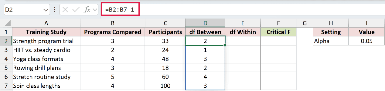
The formula subtracts one from each program count and spills into D2:D7. The strength program trial returns 2.
These range formulas spill in Excel 2021, Excel 2024, and Microsoft 365. In Excel 2019 and earlier, use per-row versions and fill them down.
Next, calculate the within-group degrees of freedom in E2:
=C2:C7-B2:B7
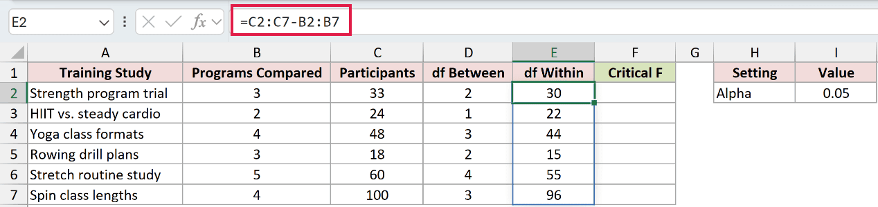
This subtracts each study’s program count from its participant count. The strength trial returns 30, while the rowing study returns 15.
Now enter the F.INV.RT formula in F2:
=F.INV.RT(I2,D2:D7,E2:E7)
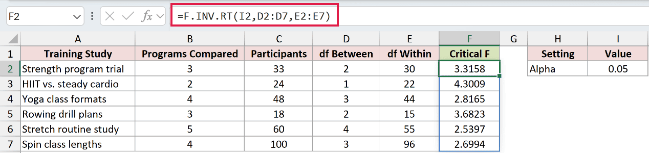
Excel pairs the degrees of freedom on each row and spills the cutoffs into F2:F7. The alpha in I2 applies to every row.
The strength trial returns 3.3158, while the rowing study returns 3.6823. Both compare 3 programs, but the strength trial has more participants and a lower cutoff.
These are thresholds for future F statistics. The design table alone doesn’t tell us whether any program performs differently.
Pro Tip: Keep the output cells below each spill formula empty. If another entry blocks the results, Excel returns #SPILL!.
Example 2: Compare ANOVA F With Its Cutoff
Now let’s calculate the statistic from actual observations before testing it.
Below is the dataset. Columns A:C hold steers’ daily weight gains under different feed rations, while E:F contains the Alpha input and labeled calculation cells.
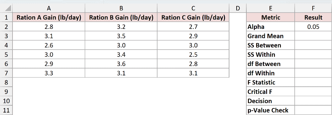
We want to test whether the ration groups have equal mean daily gains, using the alpha of 0.05 in F2.
Start with the grand mean in F3:
=AVERAGE(A2:C7)
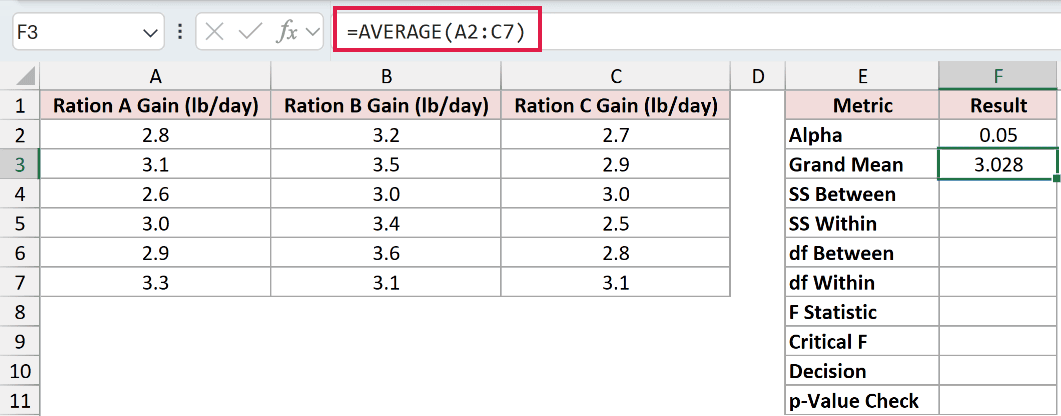
The overall mean displays as 3.028. Next, calculate the between-group sum of squares in F4:
=COUNT(A2:A7)*(AVERAGE(A2:A7)-F3)^2+COUNT(B2:B7)*(AVERAGE(B2:B7)-F3)^2+COUNT(C2:C7)*(AVERAGE(C2:C7)-F3)^2
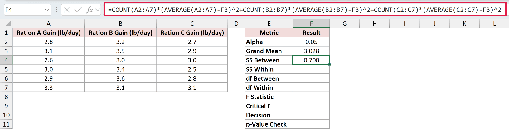
Each term measures a ration mean’s squared distance from the grand mean, weighted by its observation count. The total displays as 0.708.
Calculate the within-group sum of squares in F5:
=DEVSQ(A2:A7)+DEVSQ(B2:B7)+DEVSQ(C2:C7)
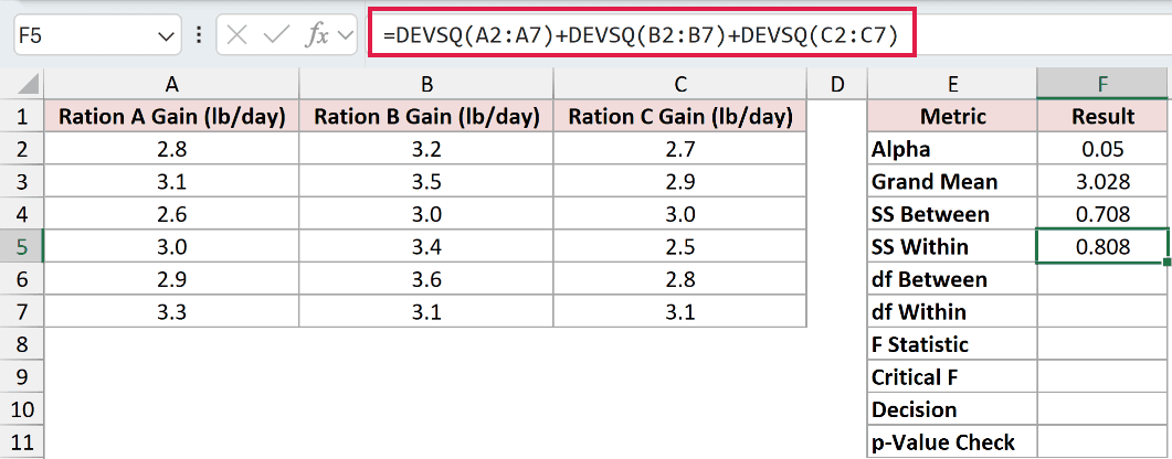
DEVSQ measures variation around each ration’s own mean. Adding those amounts returns 0.808.
For the between-group degrees of freedom, enter this in F6:
=COLUMNS(A2:C7)-1
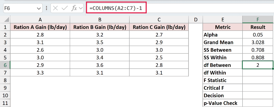
This returns 2. Calculate the within-group degrees of freedom in F7:
=COUNT(A2:C7)-COLUMNS(A2:C7)
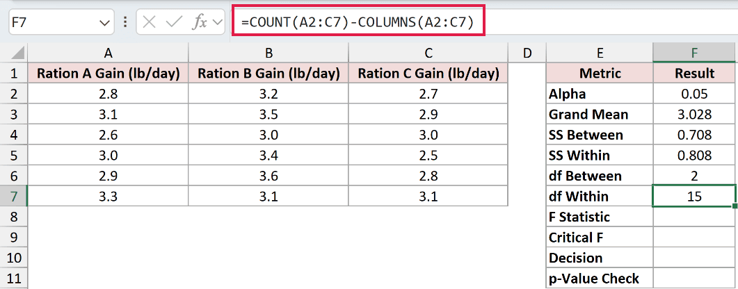
The result is 15. Now calculate F in F8:
=(F4/F6)/(F5/F7)
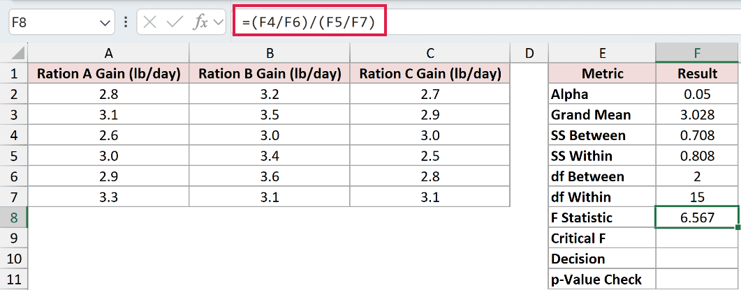
Each sum of squares is divided by its degrees of freedom. Dividing the resulting between-group mean square by the within-group mean square returns 6.567.
Use F.INV.RT in F9 to calculate the rejection cutoff:
=F.INV.RT(F2,F6,F7)
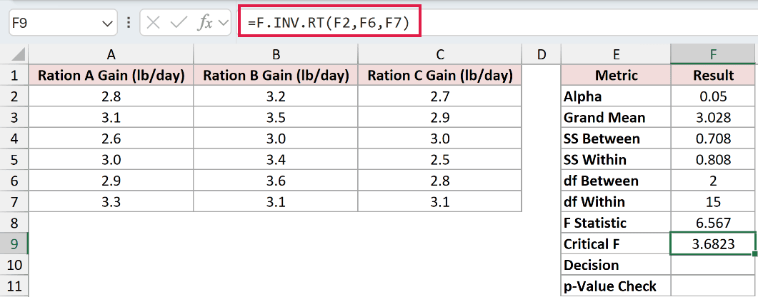
The critical value is 3.6823. Our F statistic of 6.567 is above it, so the test rejects equal means.
Make that comparison explicit in F10:
=IF(F8>F9,"Reject equal means","Fail to reject")
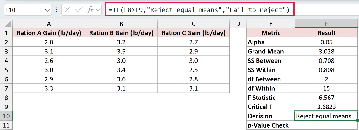
The cell returns Reject equal means. This provides evidence that at least one ration mean differs.
Finally, use F.DIST.RT in F11 as a p-value cross-check:
=F.DIST.RT(F8,F6,F7)
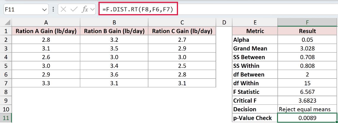
The cross-check returns 0.0089, below alpha 0.05. This p-value confirms the critical-value decision.
Example 3: Compare Different Significance Levels
The same F statistic can clear one cutoff and fall short of another.
Below is the dataset. Column A lists alpha choices; the Fertilizer Trial card holds the reported statistic, fertilizer count, plot count, and degrees-of-freedom calculation cells.
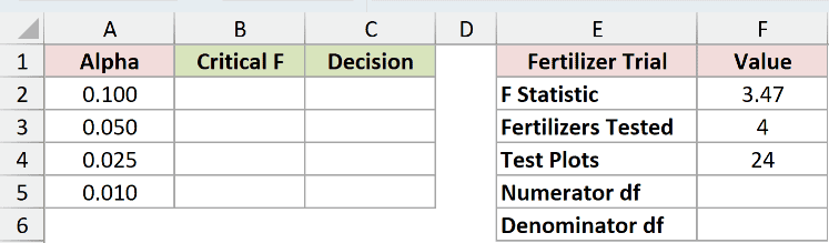
We want to compare the trial’s reported F statistic of 3.47 against the cutoff for each alpha.
Calculate the numerator degrees of freedom in F5:
=F3-1
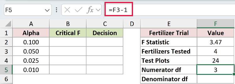
The fertilizer count produces 3 numerator degrees of freedom. Calculate the denominator degrees of freedom in F6:
=F4-F3
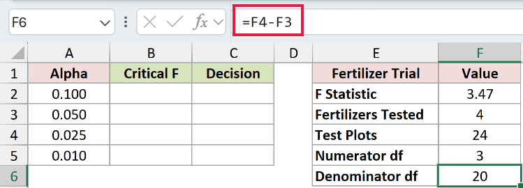
This returns 20. Enter the cutoff formula in B2:
=F.INV.RT(A2:A5,F5,F6)
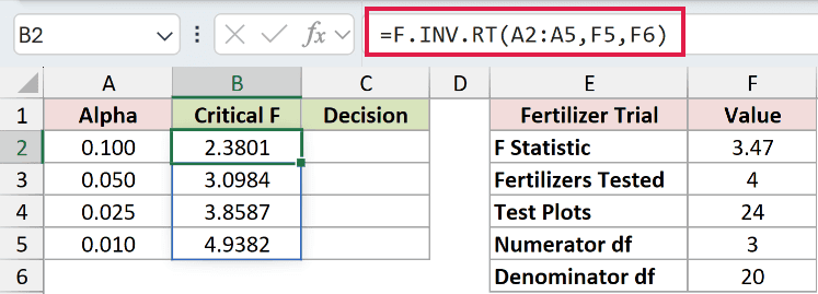
The formula spills into B2:B5. As alpha decreases, the critical F increases:
- Alpha 0.100: 2.3801.
- Alpha 0.050: 3.0984.
- Alpha 0.025: 3.8587.
- Alpha 0.010: 4.9382.
Compare the reported F with every cutoff by entering this in C2:
=IF(F2>B2:B5,"Significant","Not Significant")
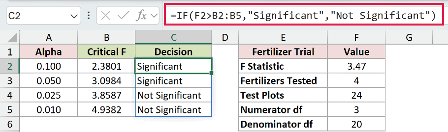
The decisions spill into C2:C5. The result is Significant at alpha 0.100 and 0.050, but Not Significant at 0.025 and 0.010.
The observations and F statistic haven’t changed. The smaller right-tail probability sets a higher threshold for rejection.
Example 4: Check a Regression Model’s Significance
For regression, we can read the F statistic from LINEST and calculate its cutoff alongside it.
Below is the dataset. It contains monthly TV, search, and email spending alongside revenue, with an Alpha input and labeled calculation cells in G:H.
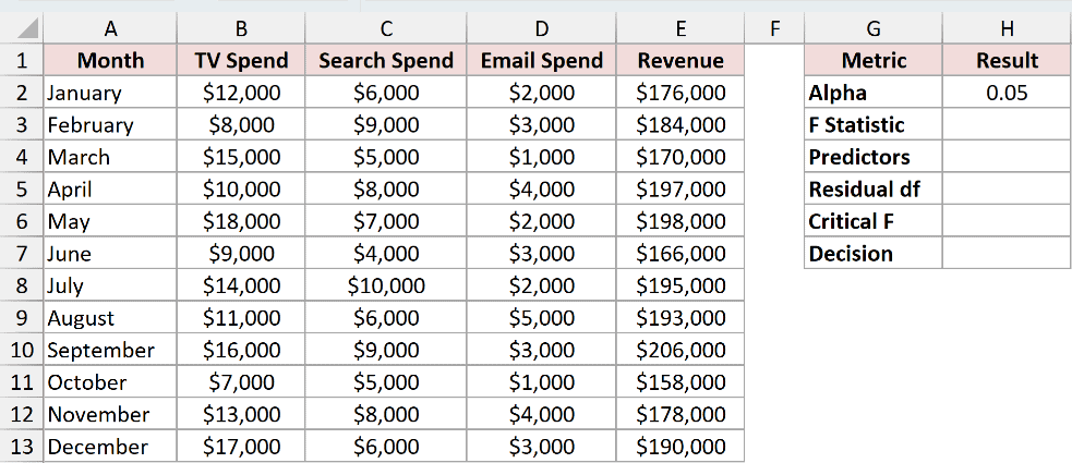
We want to test the overall regression model at the alpha of 0.05 in H2.
Extract LINEST’s F statistic into H3:
=INDEX(LINEST(E2:E13,B2:D13,TRUE,TRUE),4,1)
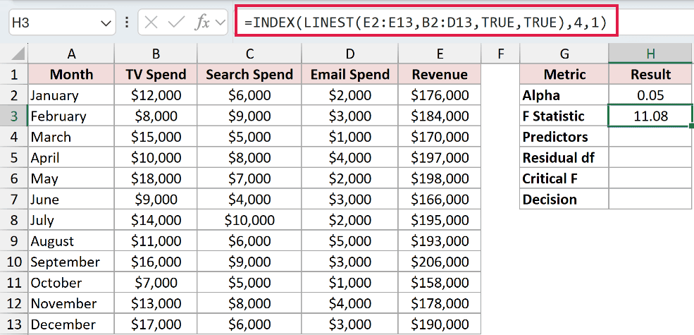
LINEST fits revenue against the spending columns and includes its statistics. INDEX selects the F statistic from that output, returning 11.08.
Count the predictors in H4:
=COLUMNS(B2:D13)
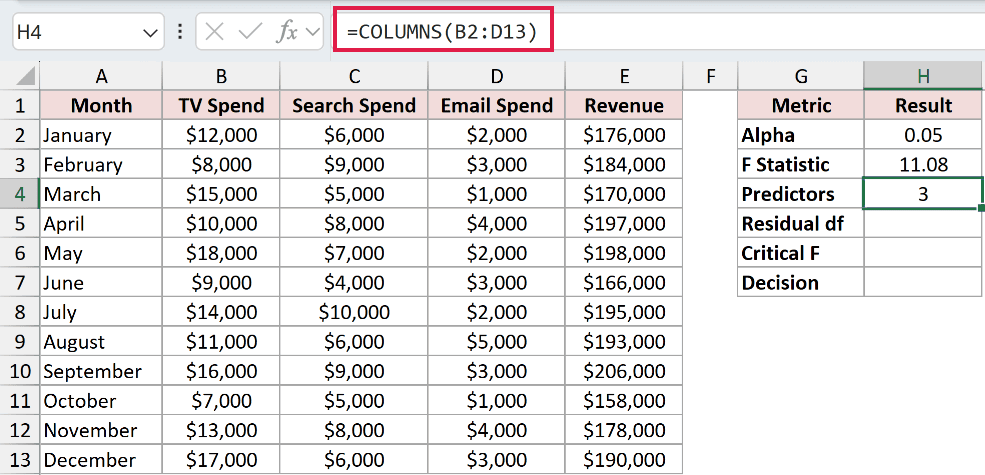
The result is 3. This predictor count is the numerator degrees of freedom for the overall F-test.
Extract the residual degrees of freedom into H5:
=INDEX(LINEST(E2:E13,B2:D13,TRUE,TRUE),4,2)
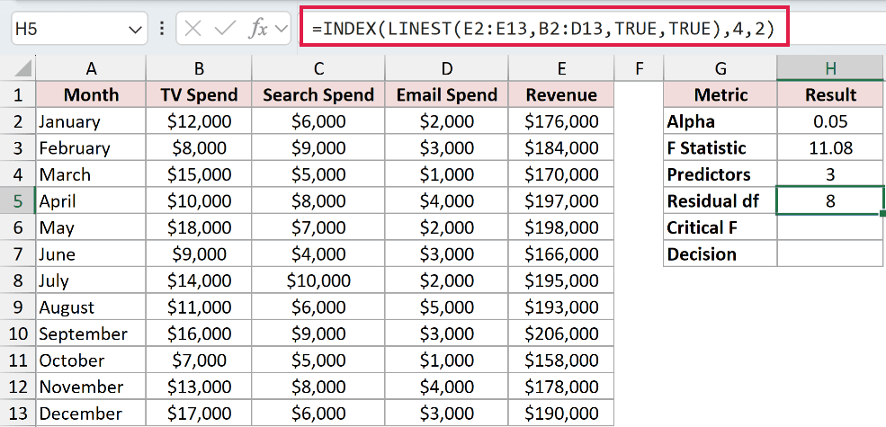
This returns 8. Both extractions use row 4 of LINEST’s statistics output, which holds F and the residual degrees of freedom.
Now calculate the critical value in H6:
=F.INV.RT(H2,H4,H5)
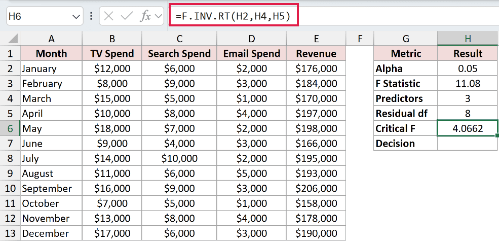
F.INV.RT returns 4.0662. Compare the model’s F statistic with that cutoff in H7:
=IF(H3>H6,"Model is significant","Not significant")
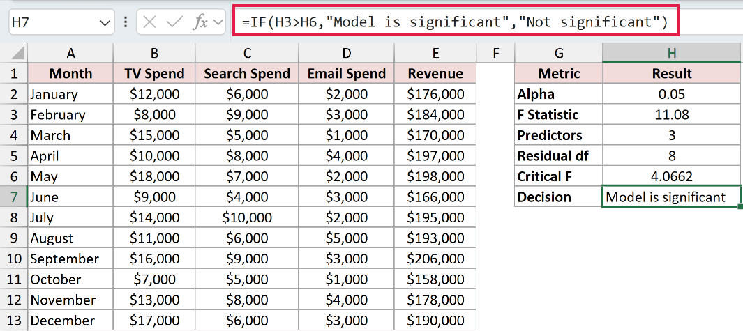
Since 11.08 exceeds 4.0662, the cell returns Model is significant. The overall test evaluates the spending channels together.
Example 5: Avoid the Two-Sided Variance Trap
A question about whether variances differ needs a different probability input from a one-direction test.
Below is the dataset. Columns A:B list independent runners’ 5K times for group runs and a solo plan, with unequal sample lengths and a labeled calculation card.
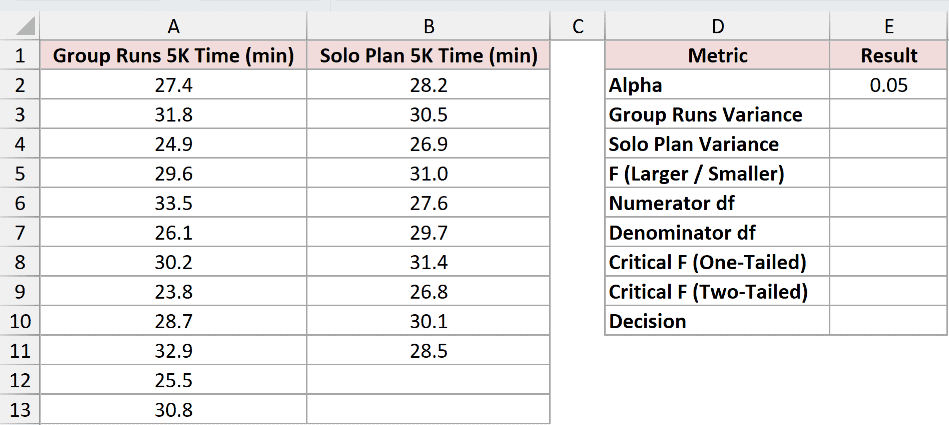
We want to test whether the time variances differ in either direction, using the alpha of 0.05 in E2.
The blank cells below the solo-plan sample reflect its shorter list. These aren’t matched pairs with missing times.
Calculate the group-runs sample variance in E3 with VAR.S:
=VAR.S(A2:A13)
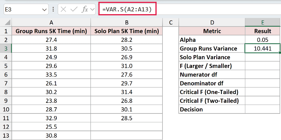
The result is 10.441. Calculate the solo-plan sample variance in E4:
=VAR.S(B2:B11)
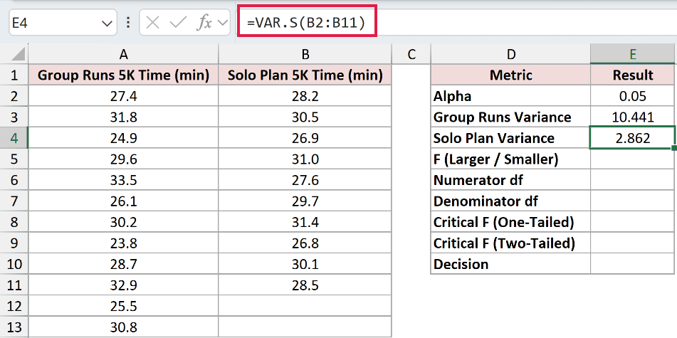
The solo-plan variance is 2.862. Put the larger variance on top to calculate F in E5:
=MAX(E3,E4)/MIN(E3,E4)
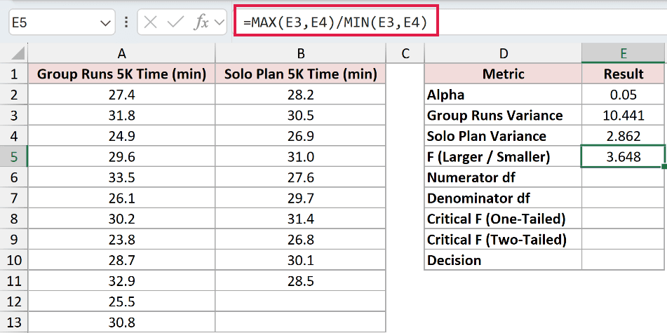
The ratio is 3.648. The group-runs variance is larger, so its sample supplies the numerator degrees of freedom.
Calculate those numerator degrees of freedom in E6:
=COUNT(A2:A13)-1
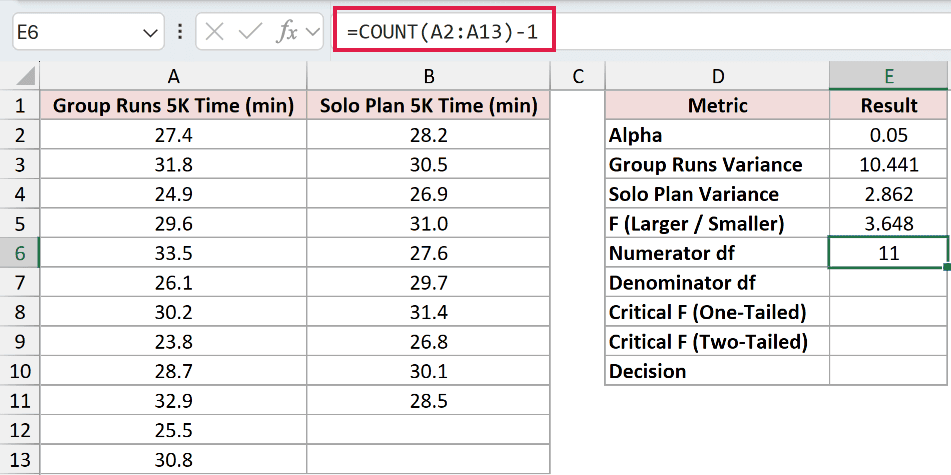
This returns 11. Calculate the denominator degrees of freedom from the solo-plan sample in E7:
=COUNT(B2:B11)-1
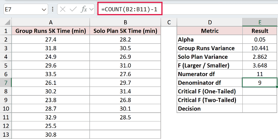
This returns 9. Keep these degrees of freedom aligned with the samples in the numerator and denominator.
The formula in E8 deliberately demonstrates the mistake: using an unsplit alpha for this two-sided question.
=F.INV.RT(E2,E6,E7)
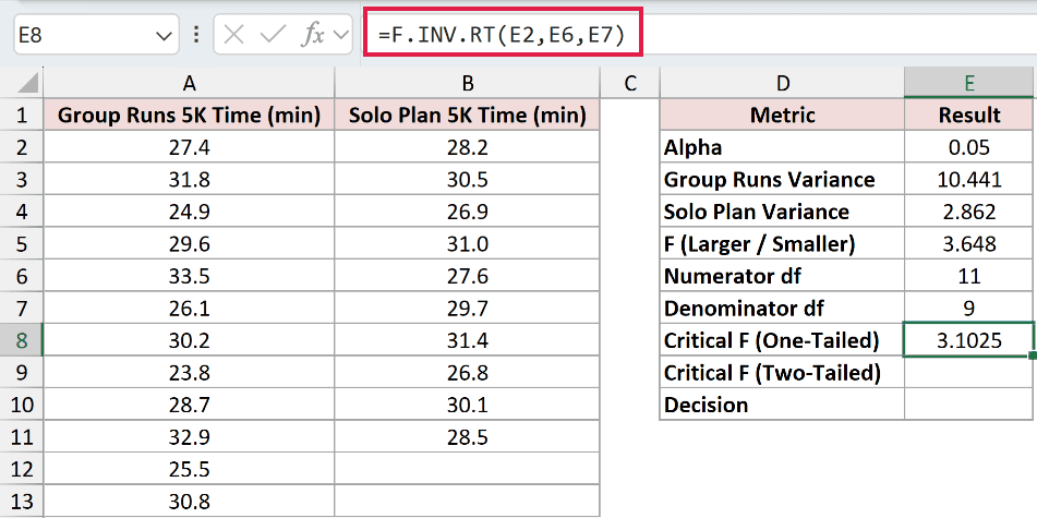
That incorrect one-tailed cutoff is 3.1025. Our F statistic clears it, but using it here would apply the wrong rejection threshold.
For the correct two-sided cutoff, split alpha across the tails. Enter this in E9:
=F.INV.RT(E2/2,E6,E7)
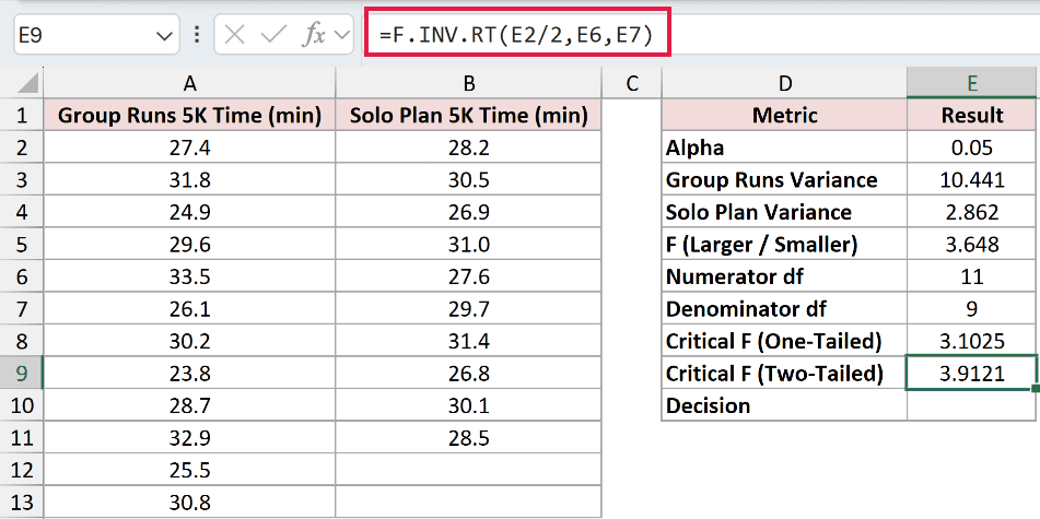
The correct upper cutoff is 3.9121. The F statistic of 3.648 falls below it, so the two-sided test doesn’t reject equal variances.
Use the correct cutoff in the decision formula in E10:
=IF(E5>E9,"Variances differ","No evidence of a difference")
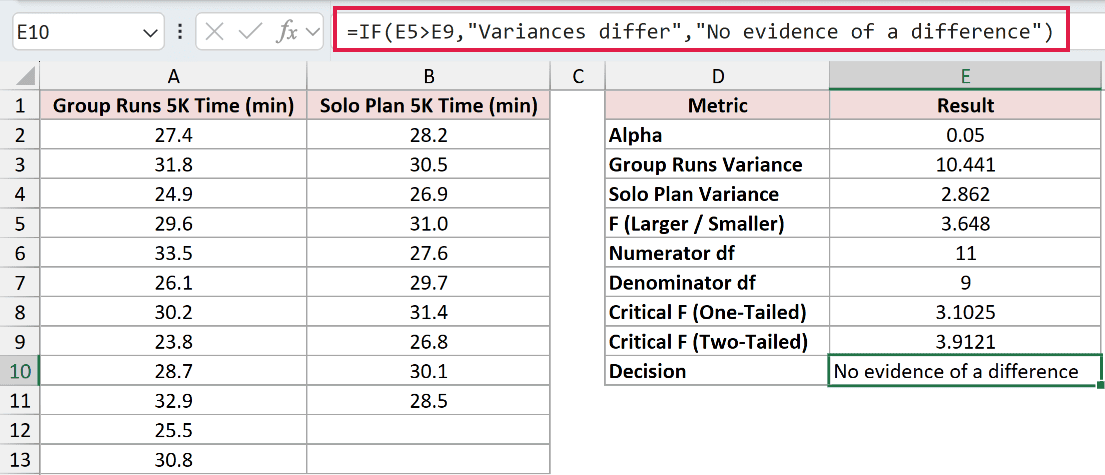
The cell returns No evidence of a difference. That doesn’t prove the variances are equal; the test hasn’t found enough evidence to reject equality.
Pro Tip: The variance-ratio formula automatically puts the larger variance on top, but these degrees-of-freedom formulas use fixed samples. If the solo-plan variance becomes larger, swap the sample references used for the numerator and denominator degrees of freedom.
Tips & Common Mistakes
- Enter alpha as a probability. Typing
5instead of0.05returns#NUM!. - Check the endpoints. A probability of
0returns#NUM!; a probability of1returns0. Degrees of freedom below1also return#NUM!. - Keep the tails straight. F.INV is the left-tail inverse. For an upper cutoff with that function, use the complementary probability instead of passing alpha directly.
- Keep degrees of freedom in order. The numerator’s degrees of freedom belong first, followed by the denominator’s. Swapping them changes the cutoff.
- Distinguish a cutoff from a p-value. F.INV.RT converts a right-tail probability into an F value. F.DIST.RT converts an F value back into a right-tail probability.
- Watch for implicit intersection. An inserted
@can reduce a range calculation to a single result. Keep the spilling formulas as shown when calculating a whole column. - Recognize the older name. FINV is the legacy name you may encounter in older workbooks.
Other Excel articles you may also like:
