
If you have a column of decimal numbers and you just want clean whole numbers, Excel gives you a few different ways to get there. The tricky part is that some methods change the actual value while one only changes how the number looks.
In this article I’ll walk through five ways to round to the nearest whole number, from the ROUND function to a formatting trick, so you can pick the one that fits what you’re doing.
Method #1: Using the ROUND Function
The ROUND function is the direct answer to this question. You give it a number and tell it how many decimal places to keep, and it rounds for you. To get a whole number, you keep zero decimal places.
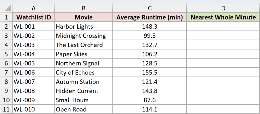
Below I have a movie watchlist. Column C has the average runtime in decimal minutes, and I want a clean whole-minute version of each one.
Here is the formula:
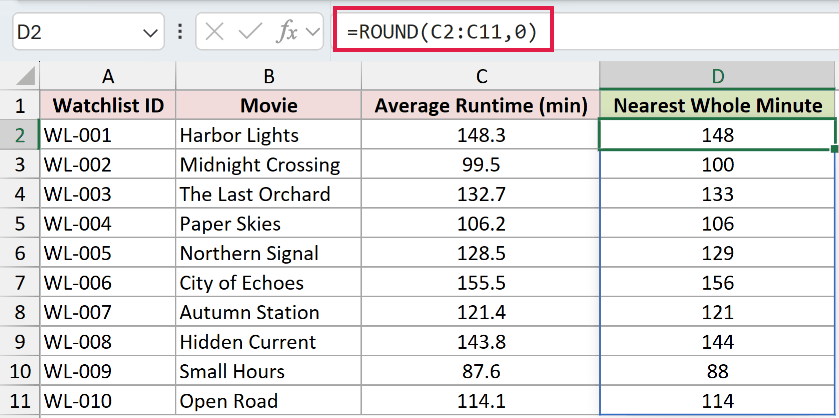
=ROUND(C2:C11,0)
How does this formula work?
ROUND takes two things: the number (or range) to round, and the number of decimal places. I passed 0 as the second argument, so every value rounds to the nearest whole number.
The .5 values round away from zero, so 99.5 becomes 100 and 128.5 becomes 129. Everything below .5 rounds down and everything above rounds up.
I gave ROUND the whole range C2:C11 in one go. In Excel 365 and Excel 2021, the formula spills down the column automatically, so you write it once in D2.
Note: If you’re on Excel 2019 or earlier, spilling isn’t available. Write =ROUND(C2,0) in D2 and copy it down the column instead.
Method #2: Using the ROUNDUP Function
Here’s a variation for when you always want to round up, no matter how small the decimal is. ROUNDUP pushes every value away from zero, so even 148.3 becomes 149.
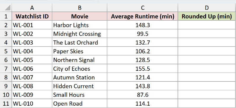
I’m using the same movie watchlist. Column C holds the decimal runtimes, and I want each one bumped up to the next whole minute.
Here is the formula:
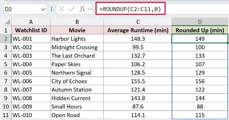
=ROUNDUP(C2:C11,0)
How does this formula work?
ROUNDUP works just like ROUND, but it ignores the usual .5 rule. Any decimal at all sends the number up to the next whole value.
So 148.3 goes to 149 and 106.2 goes to 107, even though normal rounding would leave both at 148 and 106. This is handy when you’re sizing things and can’t afford to fall short, like the number of boxes or seats you need.
In Excel 365 and Excel 2021, this range formula spills down automatically. In Excel 2019 or earlier, use =ROUNDUP(C2,0) in the first result cell and copy it down.
Method #3: Using the ROUNDDOWN Function
If you’d rather always go the other way, ROUNDDOWN is the one for you. It chops the decimal off and keeps the whole number, no matter how close you were to the next value.
Same watchlist again. Here I want every runtime pulled down to the whole minute below it.
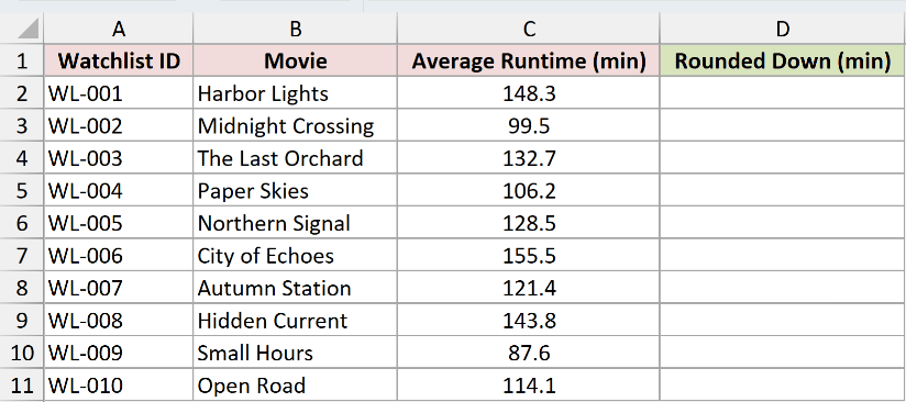
Here is the formula:
=ROUNDDOWN(C2:C11,0)
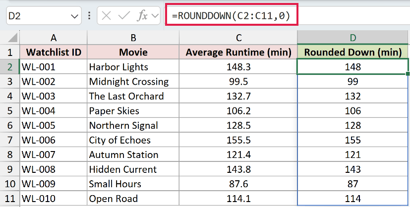
How does this formula work?
ROUNDDOWN rounds toward zero, so it always drops the decimal part. 148.3 becomes 148 and 155.5 becomes 155, even though that .5 would normally round up.
For positive numbers, =INT(C2) gives you the same result and is a bit shorter to type. The two behave differently once you go negative, though.
In Excel 365 and Excel 2021, this range formula spills down automatically. In Excel 2019 or earlier, use =ROUNDDOWN(C2,0) in the first result cell and copy it down.
Note: INT always rounds toward negative infinity, while ROUNDDOWN rounds toward zero. For -2.3, INT returns -3 but ROUNDDOWN returns -2. With all-positive numbers like these runtimes, they match exactly.
Method #4: Using the MROUND Function
MROUND rounds a number to the nearest multiple you choose. Set that multiple to 1 and you get the nearest whole number, the same as ROUND.
Here’s the watchlist once more. I’ll round column C to the nearest whole minute first, then show where MROUND really earns its place.
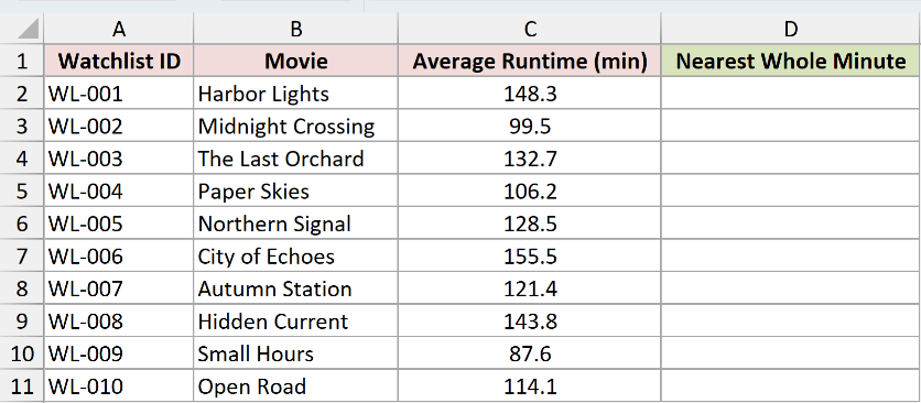
Here is the formula:
=MROUND(C2,1)
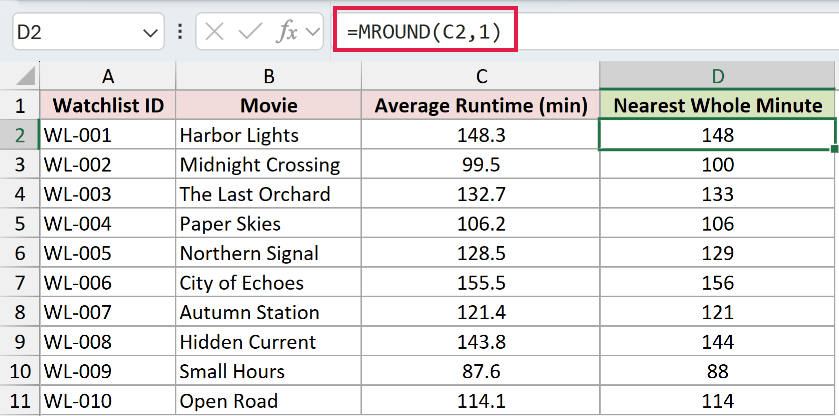
How does this formula work?
The second argument is the multiple to round to. With 1, MROUND lands on the nearest integer, so this column matches the ROUND result from Method #1 exactly.
MROUND becomes useful when you want to round to something other than 1. Say you want the nearest 5 minutes for a rough schedule. You just change the multiple.
=MROUND(C2,5)
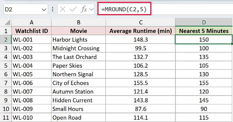
Now 148.3 rounds to 150 and 132.7 rounds to 135, snapping each runtime to the closest multiple of 5.
Enter each formula next to the first runtime and copy it down the column. Unlike ROUND, MROUND is one of Excel’s older functions that doesn’t take a whole range, so =MROUND(C2:C11,1) returns a #VALUE! error instead of spilling, even in Excel 365.
Note: MROUND returns a #NUM! error if the number and the multiple have opposite signs, for example =MROUND(-5,2). Keep both the same sign to avoid it.
Method #5: Using Format Cells (Display Only)
Sometimes you don’t want to change the value at all, you just want it to look like a whole number on screen. Formatting does exactly that. It hides the decimals without touching what’s stored in the cell.
This is the same watchlist. I want column C to show whole minutes while keeping the real decimal values underneath.
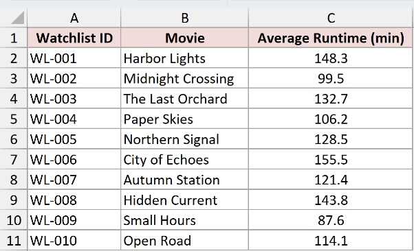
The quickest route is the Decrease Decimal button. Here are the steps:
- Select the range C2:C11.
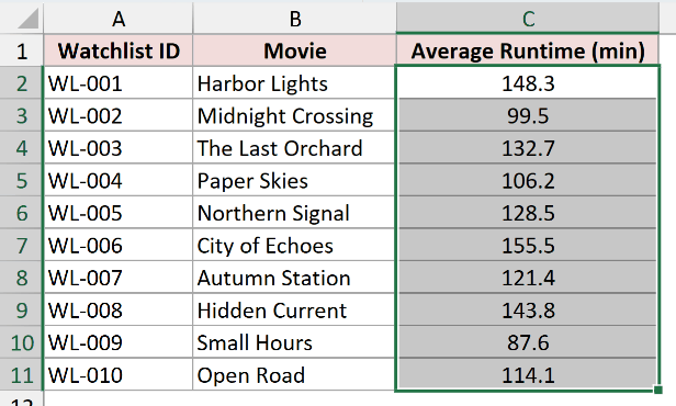
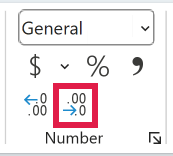
- On the Home tab, in the Number group, click the Decrease Decimal button until no decimal places are left.
You can also do this from the Format Cells dialog if you prefer setting the decimals directly:
- Select the range, press Ctrl + 1, go to the Number category, set Decimal places to 0, and click OK.
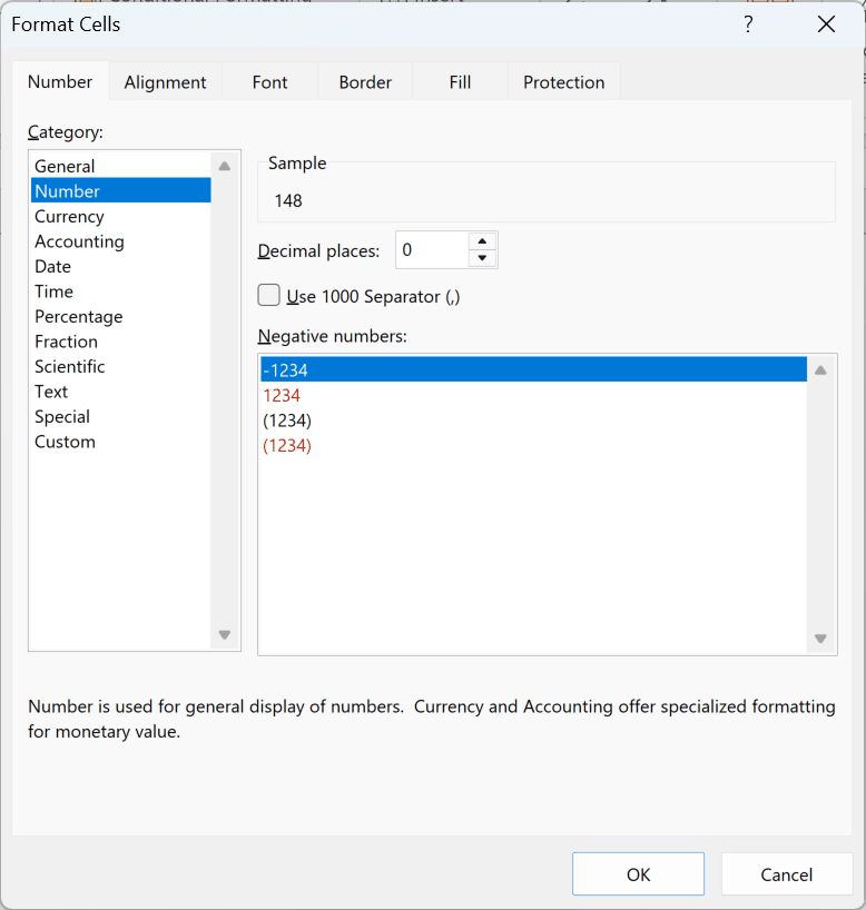
Excel applies the format and column C now shows whole numbers, while the real decimal values stay put underneath.
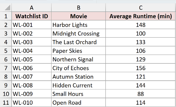
Both routes show the same whole numbers. Notice that 128.5 still displays as 129, because the display rounding follows the same away-from-zero rule as the ROUND function.
Here’s the catch. Click any of those cells and the formula bar still shows the full decimal. The cell only looks rounded.
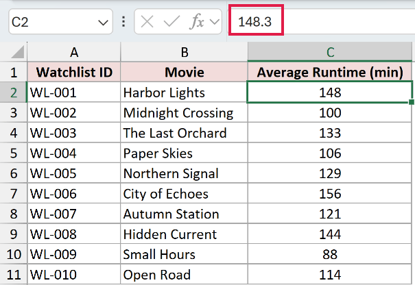
Note: Formatting changes only what you see, not the stored value. If you total a formatted column, Excel uses the full decimals, so the sum can look one or two units off from the whole numbers on screen. Use ROUND when the value itself must change.
Additional Notes About Rounding to the Nearest Whole Number in Excel
- ROUND, ROUNDUP, and ROUNDDOWN all describe direction as away from or toward zero, not simply up or down. For negative numbers this matters: ROUND(-2.5,0) gives -3, not -2.
- There’s a workbook setting under File > Options > Advanced called “Set precision as displayed.” Turning it on permanently rounds stored values to what’s shown, which can quietly change your data, so leave it off unless you really mean it.
- If your rounded numbers still show stray decimals, an outer ROUND is the fix. Wrapping a calculation like
=ROUND(A2*1.075,0)rounds the actual result rather than just its appearance. - Rounding early in a chain of calculations can nudge your final total. When accuracy matters, keep the full decimals in your working cells and round only the final figure you present.
Frequently Asked Questions
Does rounding to the nearest whole number always round .5 up?
Only for positive numbers. Excel rounds .5 away from zero, so 2.5 goes to 3 but -2.5 goes to -3. It’s “up” in size, not always up on the number line.
How do I round an entire column of formula results at once?
In Excel 365 or 2021, give ROUND the whole range, like =ROUND(C2:C11,0), and it spills down the column. In older versions, write it for the first cell and copy it down.
Why does Excel still calculate with decimals after I format a cell to show 0 decimal places?
Because formatting only hides the decimals, it doesn’t remove them. The cell still stores the full value, so any formula that references it uses the real number. To actually change the value, use ROUND.
Conclusion
Rounding to the nearest whole number in Excel usually comes down to ROUND with zero decimal places, and that’s the one I reach for by default.
Use ROUNDUP or ROUNDDOWN when you need a fixed direction, MROUND when your target is a multiple like 5 or 10, and Format Cells only when you want the look without changing the value.
Other Excel articles you may also like:
