If you want to look up a value in a table that’s laid out horizontally, where your headings run across a row instead of down a column, the HLOOKUP function is what you’re looking for.
It searches the top row of a table for a value you choose, then returns a result from a row below it. The “H” stands for horizontal, which is the only real difference from its better-known cousin VLOOKUP.
In Excel 365, you can also feed HLOOKUP a whole row of lookup values and the matching results spill across the cells automatically. I’ll show you that along with four other examples below.
HLOOKUP Function Syntax in Excel
Here is the syntax of the HLOOKUP function:
=HLOOKUP(lookup_value, table_array, row_index_num, [range_lookup])
- lookup_value: The value to find in the top row of the table.
- table_array: The table where the lookup happens. The top row is the one HLOOKUP searches.
- row_index_num: The row number to return the value from, counting down from the top of the table (row 1 is the top row itself).
- [range_lookup]: Optional. Use FALSE for an exact match, or TRUE (or leave it out) for an approximate match.
When to Use HLOOKUP Function
- When your data is arranged with headings across the top row, like months or categories spread left to right.
- When you want to pull a specific row of data for a heading you look up.
- When you need an approximate match against sorted breakpoints, like price tiers or weight bands.
- When you want to combine it with MATCH for a flexible two-way lookup.
Example 1: Basic Horizontal Lookup
Let’s start with a simple exact-match lookup.
Below is the dataset. The top row has months running across, and each row below holds a different metric: revenue, expenses, and profit.
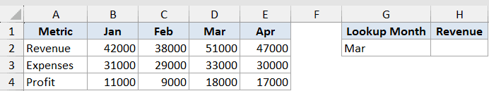
I want to find the revenue for the month typed in cell G2, which is “Mar”.
Here is the formula:
=HLOOKUP(G2,A1:E4,2,FALSE)
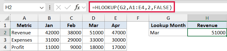
HLOOKUP searches the top row of A1:E4 for “Mar”, finds it in column D, then returns the value from row 2 of the table. That’s the revenue figure, 51,000.
The FALSE at the end forces an exact match, which is what you want almost every time you look up text.
Pro Tip: Always add FALSE as the last argument for an exact match. Leave it out and HLOOKUP switches to approximate match, which can quietly return the wrong value.
Example 2: Return a Value from a Lower Row
The row_index_num argument controls which row you pull from, so you can reach deeper into the table.
Below is the dataset. The top row lists subscription plans, and the rows below hold the monthly price, users included, and storage for each plan.
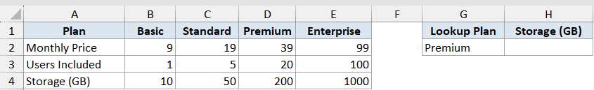
I want the storage that comes with the “Premium” plan in cell G2. Storage sits in row 4 of the table.
Here is the formula:
=HLOOKUP(G2,A1:E4,4,FALSE)
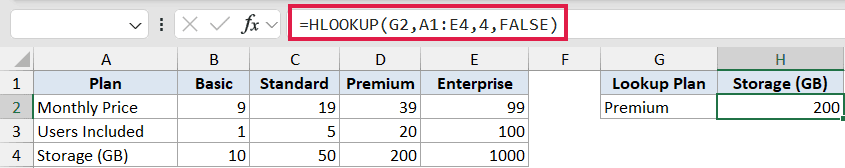
HLOOKUP finds “Premium” in the top row, then returns the value from row 4 of the table, which is 200 GB.
Just change the row number to 2 or 3 and you would get the price or the user count instead. The key is to count rows from the top of the table, not from the worksheet.
Example 3: Approximate Match for Banding
Approximate match is useful when you’re slotting a value into a range, like shipping cost by weight.
Below is the dataset. The top row holds weight breakpoints in ascending order, and the row below holds the shipping cost for each band.

I want the shipping cost for an order weight of 18 pounds, entered in cell G2.
Here is the formula:
=HLOOKUP(G2,B1:E2,2,TRUE)
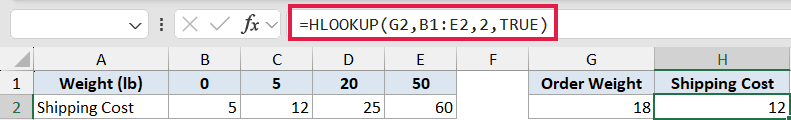
With TRUE as the last argument, HLOOKUP looks for the largest breakpoint that’s still less than or equal to 18. That’s 5, so it returns the matching cost of $12.
For approximate match to work, the top row must be sorted in ascending order. That’s why the table here starts at column B, leaving out the text label in column A.
Example 4: Two-Way Lookup with MATCH
You can make the row number dynamic by nesting the MATCH function inside HLOOKUP. This gives you a flexible two-way lookup.
Below is the dataset. The top row lists quarters and the rows below hold revenue, expenses, and profit.
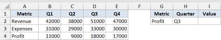
I want the figure where a chosen metric and a chosen quarter meet. Here that’s “Profit” in G2 and “Q3” in H2.
Here is the formula:
=HLOOKUP(H2,A1:E4,MATCH(G2,A1:A4,0),FALSE)
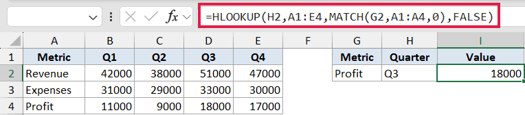
MATCH looks up “Profit” in column A and returns its position, which is 4. HLOOKUP then uses that as the row number, finds “Q3” across the top, and returns the value where they cross, 18,000.
Now you can change either the metric or the quarter and the formula adjusts on its own, with no manual row counting.
Example 5: Spill Multiple Lookups in Excel 365
In Excel 365, HLOOKUP can take a whole row of lookup values at once and spill the results.
Below is the dataset. The top row lists items with their prices in the row below, and cells G1 to I1 hold three items I want to look up.
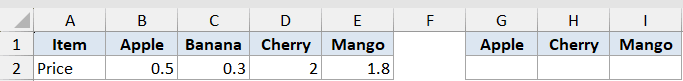
I want the prices for all three items in G1:I1 in one go.
Here is the formula:
=HLOOKUP(G1:I1,A1:E2,2,FALSE)
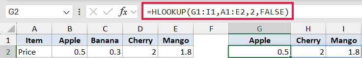
Because the lookup value is a range of three cells, HLOOKUP returns three results and spills them across G2:I2. You get 0.5, 2.0, and 1.8, one for each item.
This saves you from copying the formula across, and the results update on their own if the prices change.
Tips & Common Mistakes
- HLOOKUP can only look downward. The value you return must sit in a row below the lookup row, never above it.
- A #N/A error usually means an exact match wasn’t found. A #REF! error means your row_index_num is bigger than the number of rows in the table.
- HLOOKUP is not case sensitive, so “Mar” and “mar” are treated the same.
- In Excel 365 and 2021, the XLOOKUP function can do horizontal lookups too, with an exact match by default and no row counting. HLOOKUP is still worth knowing for older versions and for files shared with people who don’t have XLOOKUP.
HLOOKUP is the go-to function whenever your data runs across the page instead of down it. Once you’re comfortable with exact and approximate match, the MATCH trick and the 365 spill open up a lot more.
Give the examples above a try and you’ll have horizontal lookups handled.
Related Excel Functions / Articles:
- INDEX Function in Excel
- LOOKUP Function in Excel
- Using VLOOKUP Approximate Match in Excel (Examples)
- XLOOKUP Vs INDEX MATCH in Excel
- VLOOKUP Not Working – 7 Possible Reasons + Fix!
- Row vs Column in Excel – What’s the Difference?
- Find the Row Number of Matching Value in Excel
- CHOOSE Function in Excel