
The LOOKUP function in Excel searches a row or column and returns a value from the corresponding position in another row or column.
Its standard approximate-match behavior requires ascending lookup data. For an explicit exact-match search, XLOOKUP is usually easier to control.
In this article, I’ll show you how to match sorted tiers, return values from the left, and find the last entry that meets a condition.
LOOKUP Function Syntax in Excel
The LOOKUP function has two forms. The one you’ll use most often is the vector form, which searches a single row or column and returns a matching result from another.
=LOOKUP(lookup_value, lookup_vector, [result_vector])
- lookup_value: the value you want to find.
- lookup_vector: the single row or column to search in. This needs to be sorted in ascending order.
- result_vector: the single row or column to pull the result from. Optional. If you leave it out, LOOKUP returns the matching value from the lookup_vector itself.
There’s also an array form, =LOOKUP(lookup_value, array), that searches the first row or column of a block of cells and returns from the last.
Microsoft suggests using VLOOKUP, HLOOKUP, or XLOOKUP instead of the array form, so I’ll focus on the vector form here and cover the array form briefly at the end.
When to Use LOOKUP Function
- Pulling a matching value from a sorted list, like a price for a product code.
- Converting a number into a band or category, such as a score into a grade or sales into a commission rate.
- Looking up a value and returning a result from a column to its left, which VLOOKUP can’t do.
- Grabbing the last entry in a column, like the most recent balance or reading.
- Finding the latest value that matches a condition, such as the most recent price for an item.
Example 1: Vector Form Basic Lookup
Let’s start with a simple example.
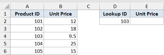
Below is the dataset. Column A has product IDs sorted in ascending order, and column B has the unit price for each one.
I want to find the unit price for product ID 103.
Here is the formula:
=LOOKUP(D2,A2:A6,B2:B6)
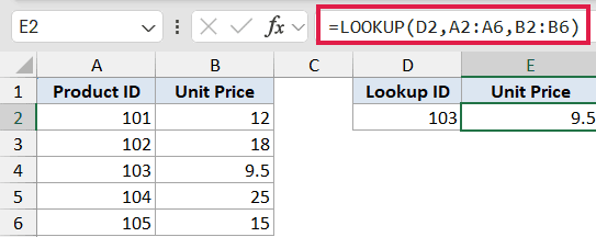
LOOKUP takes the value in D2 (103), finds it in the lookup column A2:A6, and returns the matching price from B2:B6, which is 9.5.
That’s the whole pattern: a value to find, a column to find it in, and a column to pull the result from. Just remember the lookup column needs to be sorted in ascending order for this to work reliably.
Example 2: Approximate Match With Sorted Tiers
Here’s where LOOKUP gets genuinely useful.
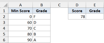
Below is the dataset. Column A has the minimum score for each grade band, sorted in ascending order, and column B has the grade letter that goes with it.
I want to find the grade for a score of 78.
Here is the formula:
=LOOKUP(D2,A2:A6,B2:B6)
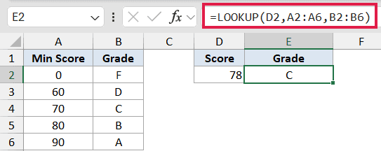
There’s no exact 78 in column A, so this is where LOOKUP’s matching behavior kicks in.
How this formula works:
- LOOKUP looks for 78 in the sorted list 0, 60, 70, 80, 90.
- It can’t find an exact match, so it settles on the largest value that is still less than or equal to 78, which is 70.
- It then returns the grade sitting next to 70, which is C.
This is why the ascending sort matters so much. LOOKUP assumes the list is sorted and walks it to find that “largest value at or below” match. If the list were out of order, you’d get the wrong answer.
Example 3: Reverse Lookup (Return a Value to the Left)
Here’s something VLOOKUP can’t do without a workaround.
Below is the dataset. Column A has salesperson names and column B has their sales figures, sorted in ascending order by sales.
I want to find which salesperson had sales of 35000.
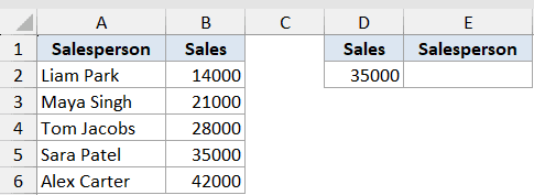
Here is the formula:
=LOOKUP(D2,B2:B6,A2:A6)
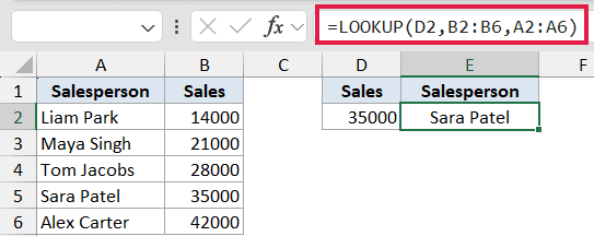
Notice the order of the ranges. The lookup column B2:B6 is to the right, and the result column A2:A6 is to its left. LOOKUP finds 35000 in column B and returns the name sitting in column A, which is Sara Patel.
VLOOKUP can only look to the right of the search column, so a left-side lookup like this would normally need INDEX and MATCH.
LOOKUP handles it directly because you tell it exactly which range to search and which range to return from.
In Excel 365, XLOOKUP can also look left without any tricks: =XLOOKUP(D2,B2:B6,A2:A6).
It doesn’t need the data sorted, so it’s the better choice if you have it. LOOKUP is still handy for older versions of Excel where XLOOKUP doesn’t exist.
Example 4: Find the Last Value in a Column
Let’s look at a popular trick that LOOKUP makes easy.
Below is the dataset. Column A has weekly dates and column B has the account balance recorded on each date.
I want to grab the most recent balance, which is the last value in column B.
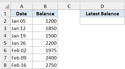
Here is the formula:
=LOOKUP(2,1/(B2:B8<>""),B2:B8)
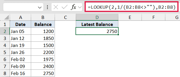
This one looks strange, so here’s what’s going on.
How this formula works:
B2:B8<>""checks each cell for content and returns TRUE for filled cells and FALSE for empty ones.- Dividing 1 by that gives a list of 1s for the filled cells (and errors for any empty ones, which LOOKUP quietly ignores).
- You then ask LOOKUP to find the value 2 in that list of 1s. Since 2 is larger than anything in the list, LOOKUP falls back to the last valid position it found.
- It returns the balance from that last position, which is 2750.
The neat part is this keeps working even when you add new rows. The formula always points at the last filled cell, so the result updates to the newest balance automatically.
Example 5: Last Value Matching a Criterion
Let’s build on that last trick with a condition.
Below is the dataset. Column A has item names, column B has the date of each entry (sorted oldest to newest), and column C has the price on that date.
I want to find the latest price for Apples, the item named in cell E2.
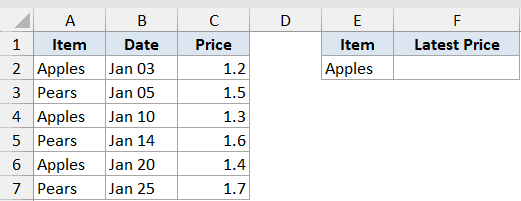
Here is the formula:
=LOOKUP(2,1/(A2:A7=E2),C2:C7)
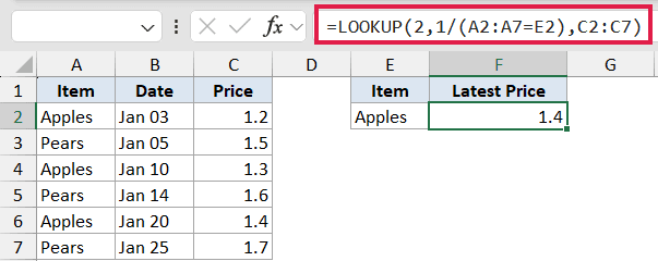
This is the same idea as the last example, just with a filter added.
How this formula works:
A2:A7=E2returns TRUE for every row where the item is Apples and FALSE everywhere else.1/(A2:A7=E2)turns those TRUEs into 1s and the FALSEs into errors that LOOKUP skips.- Searching for 2 again forces LOOKUP past the end, so it lands on the last row where the item was Apples.
- It returns the price from column C for that row, which is 1.4.
Because the data is sorted by date, the last matching row is the most recent one. That’s how you pull the latest price for any item without sorting or filtering the table yourself.
Example 6: Look Up Multiple Values at Once
Let’s finish with something you can do in Excel 365.
Below is the dataset. Column A has employee IDs sorted in ascending order and column B has each person’s department. Column D has a few IDs I want to look up at the same time.
I want to return the department for all of the IDs in D2:D5 in one go.
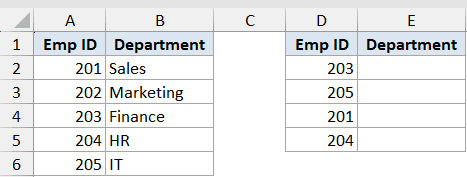
Here is the formula:
=LOOKUP(D2:D5,A2:A6,B2:B6)
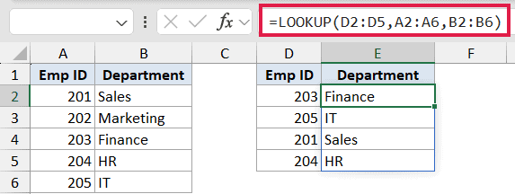
Instead of a single lookup value, I’ve handed LOOKUP the whole range D2:D5. In Excel 365 it processes each ID in turn and spills the four matching departments into the cells below, so you only write the formula once in the top cell.
You’ll see a single formula in E2 and the results filling E2:E5 on their own. If you delete the top formula, the whole spilled range disappears with it.
In Excel 365, XLOOKUP spills the same way and doesn’t need the lookup column sorted: =XLOOKUP(D2:D5,A2:A6,B2:B6). If you’re on 365, that’s usually the cleaner choice. LOOKUP is still worth knowing for older versions and for the last-value tricks above.
Tips & Common Mistakes
- Sort the lookup column in ascending order. This is the number one reason LOOKUP returns wrong answers. It assumes the search range is sorted and won’t warn you if it isn’t. If your data isn’t sorted and can’t be, use XLOOKUP or INDEX/MATCH instead.
- LOOKUP returns the closest match below, not an exact match. If the value you’re searching for is smaller than everything in the list, you’ll get a #N/A error. If it’s larger than everything, you get the last value. That fallback is exactly what powers the last-value tricks in Examples 4 and 5.
- The lookup_vector and result_vector should be the same size. If one range is longer than the other, LOOKUP can return a result from the wrong row.
- Consider XLOOKUP if you have Excel 365. XLOOKUP does everything LOOKUP does, plus exact matching by default, left lookups, and no sorting requirement. LOOKUP stays useful for older Excel versions and for the clever
=LOOKUP(2,1/(...))patterns. - The array form exists but is rarely the right tool.
=LOOKUP(lookup_value, array)searches the first row or column of a block and returns from the last. It’s there for compatibility with older spreadsheets, but VLOOKUP, HLOOKUP, or XLOOKUP give you far more control. Stick with the vector form.
LOOKUP is a small function that quietly handles a lot.
The vector form covers everyday lookups and tier or band matching, and the =LOOKUP(2,1/(...)) pattern is a genuinely useful way to grab the last value in a column or the latest entry that matches a condition.
Just keep that ascending sort rule in mind and you’ll get reliable results every time.
Related Excel Functions / Articles:
- MATCH Function in Excel
- CHOOSE Function in Excel
- IFNA Function in Excel
- SORT Function in Excel
- OFFSET Function in Excel
- SEARCH Function in Excel
- Using VLOOKUP Approximate Match in Excel (Examples)
- VLOOKUP Not Working – 7 Possible Reasons + Fix!
- INDEX Function in Excel
- Find the Closest Match in Excel (Nearest Value)
- XLOOKUP vs VLOOKUP
- Find the Last Row With Data
