
The IMPOWER function in Excel raises a complex number to a real-number power and returns the answer as complex text.
You can use whole-number powers, fractional powers for roots, or negative powers for reciprocals. The base can contain an imaginary part, but the exponent must be real.
Roots need particular care. IMPOWER selects the principal complex root, which can differ from the real root you expected for a negative number.
In this article, I’ll show you how to calculate complex powers, clean up tiny rounding residues, and interpret fractional and negative exponents.
IMPOWER Function Syntax in Excel
IMPOWER takes the complex base first and the exponent second:
=IMPOWER(inumber, number)
- inumber (required): The complex number, supplied as text such as
3+4i, a cell reference, or a result from COMPLEX. Plain real numbers also work. - number (required): The real exponent. It can be positive, negative, zero, or fractional. A number stored as text is accepted, but an imaginary exponent isn’t.
Use lowercase i or j in complex text. When entering complex text directly inside a formula, surround it with double quotes.
The result is text even when it looks like an ordinary number. For calculations that need numeric components, IMREAL, IMAGINARY, and IMABS extract numbers from it.
When to Use IMPOWER Function
- Raise complex values to powers specified in another column.
- Find principal square roots, cube roots, or other roots of complex values.
- Calculate reciprocals and reciprocal powers.
- Build a powers table and check how the magnitude changes.
Example 1: Raise Complex Numbers to Different Powers
Let’s start with a separate base and exponent on each row.
Below is the dataset. Column A contains complex or real bases, column B holds their powers, and column C will contain the results.
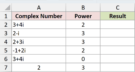
We want to raise each base to the power beside it.
Enter this formula in C2, then copy it down through C7:
=IMPOWER(A2,B2)
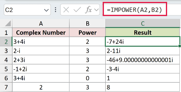
The references move with each row. Squaring 3+4i returns -7+24i, while cubing 2-i returns 2-11i.
The 2+3i row returns -46+9.00000000000001i. Those trailing digits come from floating-point rounding. We’ll handle that in the next example.
The nonzero base 3+4i raised to power 0 returns 1. The real base 2 raised to power 3 returns 8.
Both 1 and 8 are text results here. Use POWER or the ^ operator when you’re working entirely with real numbers and want numeric answers.
These are copied-down formulas by design. A bare range in either IMPOWER argument returns a single #VALUE!; the powers-table example shows an array form that works.
Example 2: Clean Up Tiny Rounding Residues
Some complex powers look untidy even when the calculation is effectively correct.
Below is the dataset. Columns A and B contain bases and powers, with separate columns for the raw result and the cleaned result.
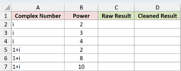
We want to calculate each power, then remove insignificant residues from its real and imaginary parts.
For the raw, noisy result, enter this in C2 and copy it through C7:
=IMPOWER(A2,B2)
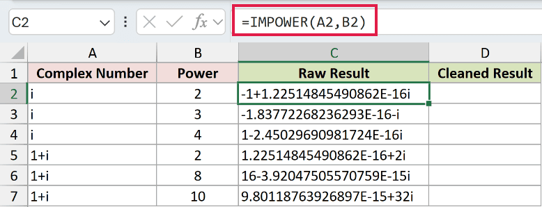
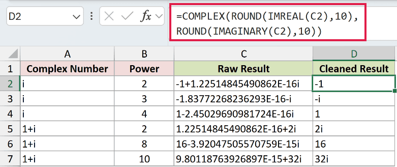
Squaring i returns -1+1.22514845490862E-16i. The imaginary part is effectively zero. The E-16 notation identifies a very small value, not an error.
Likewise, squaring 1+i returns the noisy text 1.22514845490862E-16+2i. IMPOWER calculates through magnitude and angle, which can introduce these tiny rounding residues.
For the cleanup, enter this formula in D2 and copy it through D7:
=COMPLEX(ROUND(IMREAL(C2),10),ROUND(IMAGINARY(C2),10))
How this formula works:
- IMREAL extracts the real part of the raw result as a number.
- IMAGINARY extracts the imaginary coefficient as a number.
- ROUND rounds each component separately.
- COMPLEX joins the rounded components back into complex text.
The cleaned results down column D are -1, -i, 1, 2i, 16, and 32i.
Changing the cell’s number format won’t clean up complex text. You need to extract and round its numeric components, as the formula does here.
Pro Tip: Choose rounding precision to suit your data. A genuinely small component can matter, so keep the raw result available and don’t automatically treat every small value as noise.
Example 3: Find the Principal Complex Root
Fractional exponents work, but the selected root may surprise you.
Below is the dataset. Column A contains the inputs, column B specifies the root, and columns C and D are reserved for the root and its reverse check.
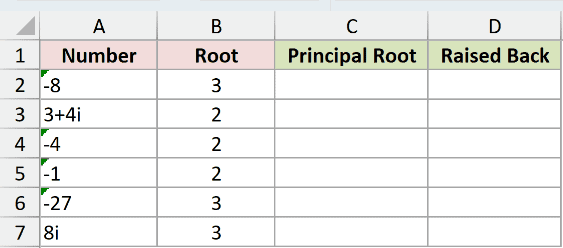
We want each principal root, then a check that raising it back recovers the original input within rounding accuracy.
Enter this in C2 and copy it through C7:
=IMPOWER(A2,1/B2)
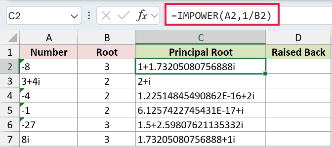
Dividing by the root number creates the fractional exponent. For the cube root of -8, Excel returns 1+1.73205080756888i, not -2.
That’s the principal complex root, selected using the base’s principal angle. IMPOWER returns that selected root rather than a list of every possible root.
The square root of 3+4i returns 2+i. IMSQRT is a more direct choice when you only need square roots.
For the reverse check, enter this in D2 and copy it through D7:
=IMPOWER(C2,B2)
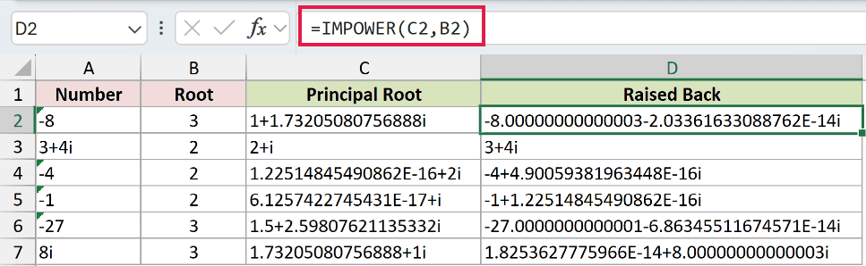
This raises the selected root to the original root number. The 2+i result returns to 3+4i exactly as displayed.
The first check displays -8.00000000000003-2.03361633088762E-14i. It’s close to the original -8, with small rounding residues in both components.
The Raised Back column is a verification step, not another root. Don’t read its tiny imaginary residue as evidence that the principal root is wrong.
Example 4: Calculate Reciprocals With Negative Powers
A negative exponent lets you calculate a reciprocal without leaving the complex-number functions.
Below is the dataset. Column A holds complex inputs; the remaining columns provide spaces for reciprocals, an IMDIV comparison, their difference, and reciprocal squares.
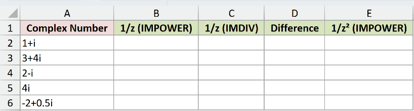
We want the reciprocal of each input and a numeric check against the equivalent IMDIV calculation.
Enter this in B2 and copy it through B6:
=IMPOWER(A2,-1)
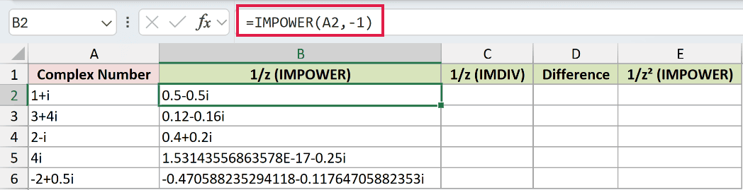
The exponent -1 calculates the reciprocal. For 1+i, the result is 0.5-0.5i.
For the IMDIV comparison, enter this in C2 and copy it through C6:
=IMDIV(1,A2)
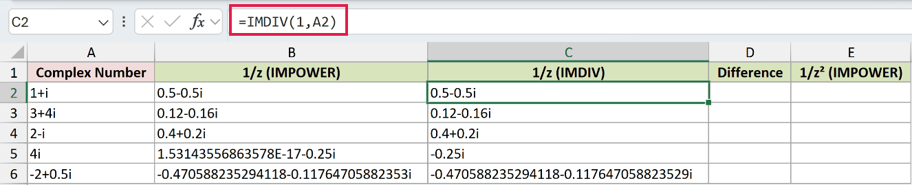
The comparison returns the same displayed text for 1+i, 3+4i, and 2-i. But the strings don’t match on every row.
For 4i, IMPOWER returns 1.53143556863578E-17-0.25i, while the IMDIV comparison returns -0.25i. A direct text-equality comparison would mistake rounding noise for a meaningful disagreement.
To measure the difference numerically, enter this in D2 and copy it through D6:
=IMABS(IMSUB(B2,C2))
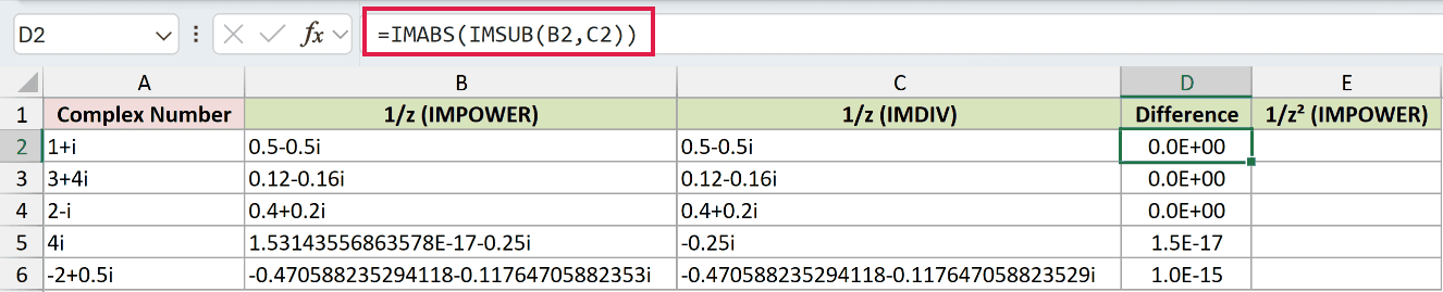
IMSUB subtracts the complex results, and IMABS returns the magnitude of that difference as a real number.
The Difference column shows 0.0E+00 for 1+i, 3+4i, and 2-i; 1.5E-17 for 4i; and 1.0E-15 for -2+0.5i.
Those last differences are tiny. Compare their size against the precision your calculation needs instead of testing whether the complex text strings are identical.
For reciprocal squares, enter this in E2 and copy it through E6:
=IMPOWER(A2,-2)

The exponent -2 calculates the reciprocal of the square. For 3+4i, it returns -0.0112-0.0384i; for 2-i, it returns 0.12+0.16i.
Example 5: Spill a Table of Powers
Now let’s calculate successive powers from a single base.
Below is the dataset. Column A lists the powers, F2 holds the typed base, and columns B through D will hold results and magnitude checks.
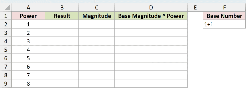
We want a spilled powers column and a check that each result’s magnitude follows the base magnitude raised to that power.
Enter this formula once in B2:
=IMPOWER(F2,SEQUENCE(8))
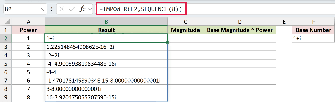
SEQUENCE generates exponents from 1 through 8. IMPOWER uses the base 1+i in F2 and spills the results into B2:B9.
Column A contains typed labels, not the exponents supplied to IMPOWER. Keep those labels aligned with the sequence if you change the table.
This spill works in Excel 2021, Excel 2024, and Microsoft 365. In Excel 2019 and earlier, use a per-row IMPOWER formula and fill it down.
The third power returns -2+2i. The eighth power returns 16-3.92047505570759E-15i, including the small imaginary rounding residue.
For the result’s magnitude, enter this in C2 and copy it through C9:
=IMABS(B2)
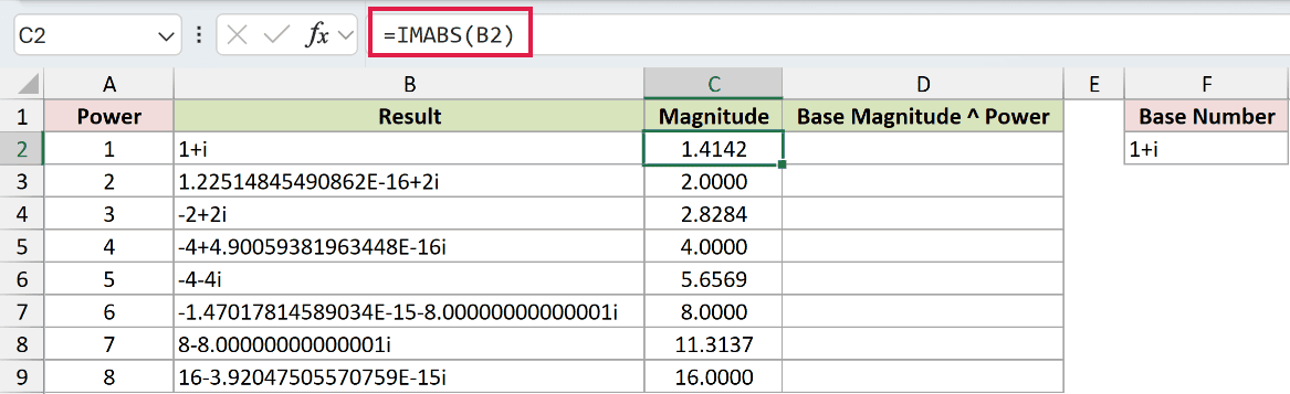
IMABS converts each complex result into a numeric magnitude. The first magnitude displays as 1.4142, and the last displays as 16.0000.
For the independent magnitude comparison, enter this in D2 and copy it through D9:
=IMABS($F$2)^A2
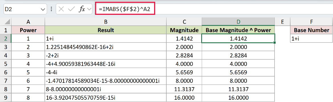
The absolute reference keeps the base fixed. This comparison raises its numeric magnitude to each power listed in column A.
Columns C and D agree at the displayed precision throughout. For example, the third power shows 2.8284 in both columns, and the eighth shows 16.0000.
Pro Tip: A bare exponent range fails, but the array generated by SEQUENCE works. A unary plus applied to a range also makes IMPOWER spill. Keep the output cells empty so the results have room.
Example 6: Understand Errors and Accepted Inputs
Finally, let’s separate invalid inputs from cases that Excel accepts quietly.
Below is the dataset. Each row names an input case, supplies a base and power, and reserves column D for the result or deliberate error.
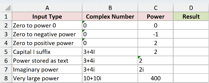
We want to see which input combinations work and why the others fail.
Enter this in D2 and copy it through D8:
=IMPOWER(B2,C2)
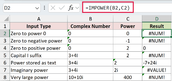
The error cells are deliberate demonstrations. Here’s what each row tells you:
- D2, zero to power zero: Returns
#NUM!. The nonzero-base rule for power zero doesn’t extend to a zero base. - D3, zero to a negative power: Returns
#NUM!because the reciprocal would require division by zero. - D4, zero to a positive power: Returns the text
0. This is an accepted input, not an error. - D5, capital I suffix:
3+4Ireturns#NUM!. Use lowercaseiorjfor the imaginary suffix. - D6, power stored as text: The text exponent
2is accepted, returning-7+24i. Numeric text alone isn’t a problem here. - D7, imaginary power: The exponent
2ireturns#VALUE!. IMPOWER accepts a complex base, but its exponent must be real. - D8, very large power: Raising
10+10ito400returns#NUM!because the result overflows Excel’s numeric capacity.
Tips & Common Mistakes
- Use the right output type. IMPOWER returns complex text. For ordinary real-number powers, use POWER or
^; for numeric components of complex results, use IMREAL or IMAGINARY. - Keep the suffix lowercase. Both
iandjwork, and IMPOWER keepsjin its output. A capitalIcauses an error. - Choose roots deliberately. A fractional exponent returns the principal complex root. It doesn’t list all roots or promise the real root of a negative base.
- Compare numeric differences. Use the IMABS and IMSUB check from Example 4 rather than equality between complex text strings. Equivalent routes can differ in their last digits.
- Don’t hide input problems automatically. Inspect the base, exponent, and suffix before adding IFERROR. A suppressed error won’t tell you whether the issue was invalid text or overflow.
- Use IMPRODUCT for multiplication. IMPOWER is useful when the operation is expressed as a power; IMPRODUCT handles multiplication of complex factors directly.
I hope you found this article helpful.
Related Excel Functions / Articles:
