IMPRODUCT Function in Excel

The IMPRODUCT function in Excel returns the product of complex numbers written in x+yi or x+yj form.

It works with complex numbers stored in cells, typed directly in a formula, or supplied through a range. The result is another complex number.

The PRODUCT function handles ordinary numbers. IMPRODUCT is the corresponding choice when the values use Excel’s complex-number text format.

In this article, I’ll show you how to multiply paired values, combine a range, build j-form inputs, and include only approved records.

IMPRODUCT Function Syntax in Excel

The syntax of the IMPRODUCT function is:

=IMPRODUCT(inumber1, [inumber2], ...)

• inumber1 is the first required complex number or range.
• [inumber2] is an additional complex number or range. IMPRODUCT accepts up to 255 arguments in total.
• Complex numbers can use the i or j suffix, but all inputs in one calculation must use the same suffix.

When to Use IMPRODUCT Function

• Multiply two or more complex numbers stored in separate cells.
• Combine every complex factor in a range into one result.
• Multiply complex values created from separate real and imaginary coefficients.
• Calculate one product for each pair of values in two lists.
• Restrict the multiplication to rows that meet a condition.

Example 1: Multiply Paired Complex Numbers With MAP

We’ll begin by multiplying two complex gains for each channel.

Below is the dataset with a base gain, an adjustment factor, an empty result column, and a scalar check for Channel A.

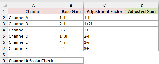
I want Excel to calculate all six pairwise products with one spilling formula.

Here is the formula entered in D2:

=MAP(B2:B7,C2:C7,LAMBDA(base_gain,adjustment_factor,IMPRODUCT(base_gain,adjustment_factor)))

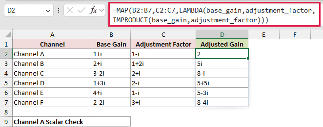
How this formula works:

• MAP moves through B2:B7 and C2:C7 together.
• LAMBDA names the current pair base_gain and adjustment_factor.
• IMPRODUCT multiplies each pair and returns 2, 5i, 8-i, 5+5i, 5-3i, and 8-4i in D2:D7.

MAP is available in Microsoft 365 and Excel 2024. The results spill from D2, so the cells below it must remain empty.

The scalar calculation in B9 checks the first spilled result separately.

Here is the scalar check formula entered in B9:

=IMPRODUCT(B2,C2)

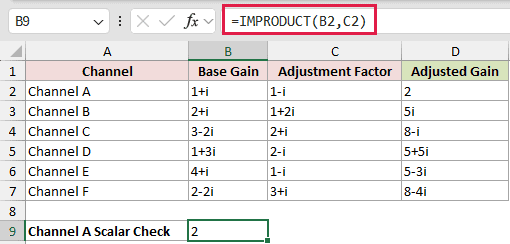
The formula multiplies 1+i by 1-i and returns 2, matching the first result from the MAP formula.

Pro Tip: If another value blocks the output range, the MAP formula returns #SPILL!. Clear the occupied cells below D2 and recalculate.

Example 2: Multiply a Range of Complex Numbers

Here is a single-result calculation across several signal stages.

Below is the dataset with five complex gains and an empty cell for the net signal gain.

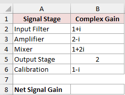
I want to multiply all five values in B2:B6 and return one combined gain.

Here is the formula entered in B8:

=IMPRODUCT(B2:B6)

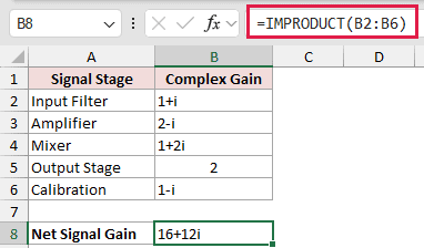
IMPRODUCT treats the range as the set of complex numbers to multiply. The formula returns 16+12i in B8.

This example also shows why IMPRODUCT is a reducer. Even though the formula receives five cells, it returns one result rather than spilling five products.

Example 3: Build j-Form Numbers With COMPLEX

Sometimes the real and imaginary coefficients begin in separate columns.

Below is the dataset with both coefficients, an empty Complex Factor column, and an empty cell for the combined factor.

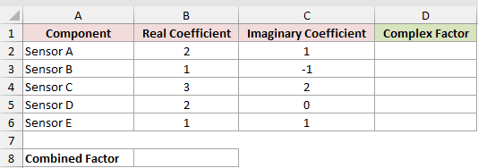
I want to create each j-form complex factor first, then multiply the completed range.

Here is the formula entered in D2 and filled down to D6:

=COMPLEX(B2,C2,"j")

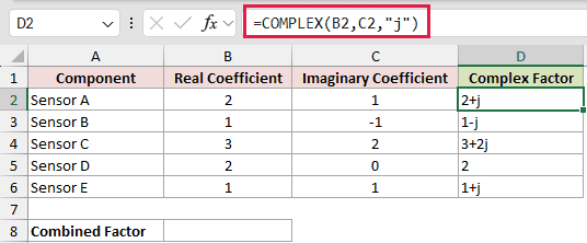
COMPLEX joins the real coefficient in column B with the imaginary coefficient in column C. The third argument tells Excel to use j as the suffix.

The formulas return 2+j, 1-j, 3+2j, 2, and 1+j in D2:D6.

Now I can multiply the completed factors in column D.

Here is the formula entered in B8:

=IMPRODUCT(D2:D6)

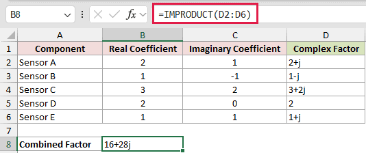
The formula returns 16+28j in B8. Because the complex inputs use j, IMPRODUCT keeps j in the result.

Pro Tip: Use lowercase i or j, and keep the suffix consistent across every complex number in the calculation.

Example 4: Multiply Only Approved Complex Factors

This example adds a condition before the multiplication.

Below is the dataset with batch names, review statuses, complex factors, and an empty cell for the approved product.

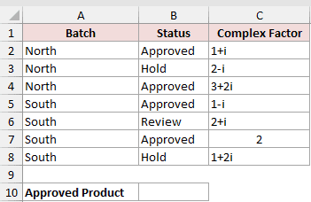
I want to multiply only the factors from rows marked Approved.

Here is the formula entered in B10:

=IMPRODUCT(FILTER(C2:C8,B2:B8="Approved"))

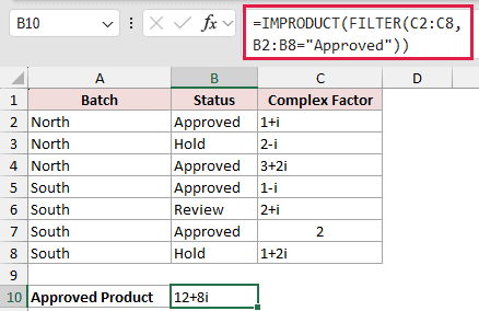
FILTER returns the factors from rows where column B contains Approved. IMPRODUCT then multiplies that filtered array and returns 12+8i in B10.

FILTER is available in Excel 2021, Excel 2024, and Microsoft 365. If no status matches, this exact formula returns a #CALC! error because [if_empty] is omitted.

Tips & Common Mistakes

• Put complex numbers typed directly into a formula inside quotation marks, such as =IMPRODUCT("1+i","1-i"). Cell references do not need quotation marks.
• Use lowercase i or j. Uppercase suffixes are not valid for Excel’s complex-number functions.
• Keep the suffixes consistent. Do not mix an i value with a j value in the same IMPRODUCT calculation.
• IMPRODUCT returns one combined result for a range. Use MAP when you need a separate product for each pair of rows.
• Check the source cells if Excel returns an error. Each complex number must follow the x+yi or x+yj text form that Excel recognizes.

I covered pairwise multiplication, range reduction, j-form inputs, and filtered multiplication with IMPRODUCT.

I hope you found this article helpful.

List of All Excel Functions

Other Excel articles you may also like:

• IMSUM Function in Excel
• COMPLEX Function in Excel
• IMDIV Function in Excel
• IMABS Function in Excel
• Excel IMCONJUGATE function
• IMPOWER function