IMSECH Function in Excel (4 Easy Examples)

The IMSECH function in Excel returns the hyperbolic secant of a complex number. This is the reciprocal of its hyperbolic cosine.

Excel stores the answer as text, including both real and imaginary parts when needed. That matters when you compare results or use them in another calculation.

I’ll show you how to calculate complex hyperbolic secants, check the reciprocal relationship, and recognize large-input behavior and unexpected blank-cell results.

Table of Contents

IMSECH Function Syntax in Excel

IMSECH takes one required argument:

=IMSECH(inumber)

inumber (required): The complex number to evaluate, supplied as a cell reference, a real number, or complex text in x+yi or x+yj form.

Use lowercase i or j for the imaginary suffix. COMPLEX can build the input when your real and imaginary parts occupy separate cells.

IMSECH is available in Excel 2013 and later.

When to Use IMSECH Function

Calculate the hyperbolic secant of complex values already stored in a worksheet.
Check a reciprocal calculation involving IMCOSH and IMDIV.
Examine how the result behaves as the real input grows.
Identify invalid complex inputs and blank cells that silently produce an answer.

Example 1: Calculate Complex Hyperbolic Secants

Let’s start with a column containing complex numbers in both supported suffix styles.

Below is the dataset. Column A holds complex inputs, column B will hold their hyperbolic secants, and column C will hold the magnitudes.

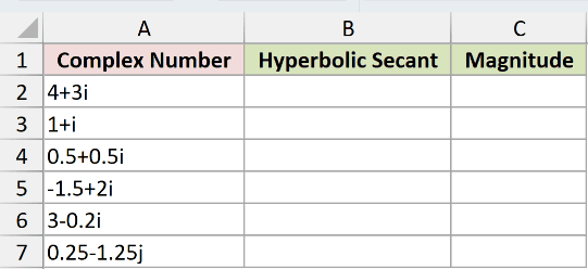
We want each input’s hyperbolic secant and a numeric measure of the result’s size.

Enter this formula in B2 and copy it down to B7:

=IMSECH(A2)

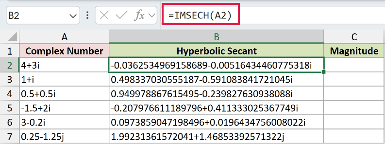
For 4+3i, B2 returns -0.0362534969158689-0.00516434460775318i. The result contains both a real part and an imaginary part.

The input 0.25-1.25j returns 1.99231361572041+1.46853392571322j. Notice that Excel keeps the lowercase j suffix.

These are text results, so changing the number format won’t shorten their decimal places.

To calculate a numeric magnitude, enter this formula in C2 and copy it down to C7:

=ROUND(IMABS(B2),4)

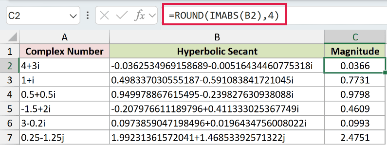
IMABS converts the complex result into its magnitude, and ROUND rounds that number. C2 displays 0.0366, while C7 displays 2.4751.

We’re copying formulas down throughout this workbook. Passing a bare range directly to IMSECH returns a single #VALUE! instead of a column of answers.

Example 2: Check the Reciprocal Without Comparing Text

The reciprocal relationship works, but an exact text comparison can make matching calculations look inconsistent.

Below is the dataset. Column A holds complex inputs, and columns B through F will hold the calculations and comparisons.

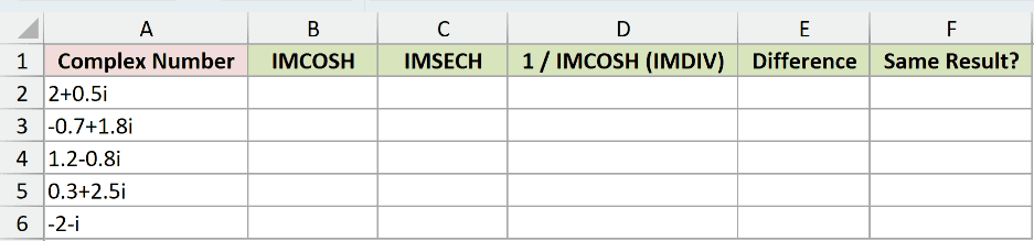
We want to compare IMSECH with the reciprocal of IMCOSH and measure any numerical difference.

First, calculate the supporting hyperbolic cosine in B2 and copy down to B6:

=IMCOSH(A2)

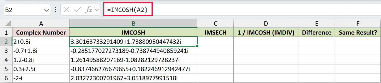
For 2+0.5i, this returns 3.30163733291409+1.73880950447432i.

Enter the direct IMSECH calculation in C2 and copy down to C6:

=IMSECH(A2)

C2 returns 0.237113896015908-0.124876191556598i.

For the reciprocal comparison, enter this formula in D2 and copy down to D6:

=IMDIV(1,B2)

IMDIV divides by the complex hyperbolic cosine. The comparison in D2 returns 0.237113896015908-0.124876191556598i, matching C2 exactly on this row.

Now measure the numerical difference in E2 and copy down to E6:

=IMABS(IMSUB(C2,D2))

IMSUB subtracts the complex results, then IMABS measures the size of that difference.

E2 and E3 display 0.0E+00. E4 through E6 display 1.0E-15, a tiny rounding difference that is effectively zero for this comparison.

For the misleading text-comparison demonstration, enter this formula in F2 and copy down to F6:

=C2=D2

The text comparison returns TRUE for 2+0.5i and -0.7+1.8i. It returns FALSE for 1.2-0.8i, 0.3+2.5i, and -2-i.

Those FALSE results reflect differences in the final text digits. They don’t disprove the reciprocal relationship.

Pro Tip: Read 1.0E-15 in the Difference column as a tiny rounding difference, not a large gap between the answers.

Example 3: Compare Large Real Inputs

For the largest real inputs here, IMSECH returns the text 0 while IMCOSH returns #NUM!.

Below is the dataset. Column A contains real inputs, column B will show IMSECH results, and column C provides the IMCOSH comparison.

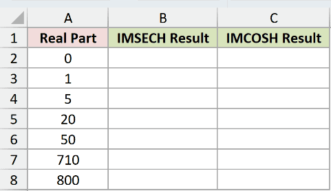
We want to see the secant shrink while the comparison hyperbolic cosine grows.

Enter this formula in B2 and copy down to B8:

=IMSECH(A2)

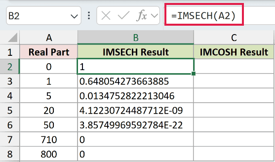
At input 20, IMSECH returns 4.12230724487712E-09. At 50, it returns 3.85749969592784E-22. These are very small values written in scientific notation.

At 710 and 800, IMSECH returns the text 0 without an error. Don’t interpret this computed zero as proof that the mathematical value is exactly zero.

For the IMCOSH comparison, enter this formula in C2 and copy down to C8:

=IMCOSH(A2)

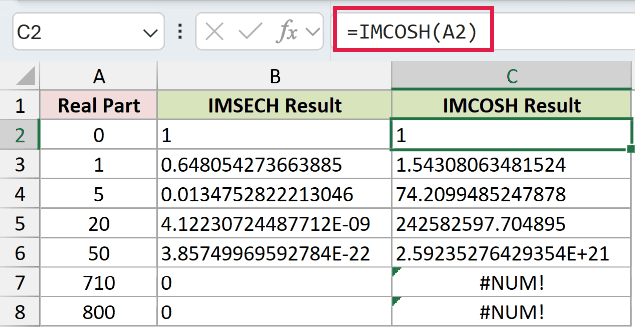
The comparison reaches 2.59235276429354E+21 at input 50. At 710, comparison cell C7 returns #NUM! because IMCOSH overflows.

At 800, comparison cell C8 also returns #NUM! from overflow. Both errors are deliberate demonstrations, while IMSECH returns 0 on those rows.

Using IMSECH directly avoids calculating IMCOSH first, so you sidestep its overflow error.

Example 4: Recognize Input Errors and Blank Cells

An unexpected answer can come from the input rather than the calculation.

Below is the dataset. Column A labels each input type, column B contains the test inputs, and column C will hold the results or deliberate errors.

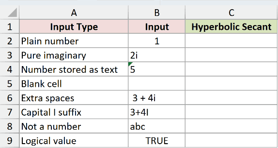
We want to identify accepted inputs, invalid suffixes, and the silent blank-cell trap.

Enter this formula in C2 and copy down to C9:

=IMSECH(B2)

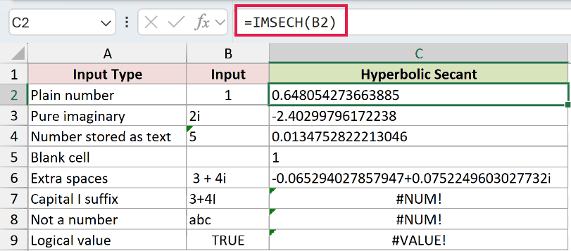
Here’s what each row shows:

Plain number, B2: The input 1 is accepted, and C2 returns the text 0.648054273663885.
Pure imaginary, B3: The input 2i is accepted, and C3 returns the text -2.40299796172238 without an imaginary suffix.
Number stored as text, B4: The text input 5 is accepted, and C4 returns 0.0134752822213046.
Blank cell, B5: Excel treats the empty input as zero, so C5 silently returns the text 1. This is the missing-input trap.
Extra spaces, B6: The spaced complex input is accepted. C6 returns -0.065294027857947+0.0752249603027732i; spaces aren’t the cause of an error here.
Capital I suffix, B7: C7 deliberately returns #NUM! because the suffix is uppercase. Change the suffix to lowercase.
Not a number, B8: C8 deliberately returns #NUM! because abc isn’t a valid complex number. Replace it with a valid input.
Logical value, B9: C9 deliberately returns #VALUE! because TRUE isn’t an accepted argument. Supply the intended numeric or complex value.

Pro Tip: Check for missing inputs before trusting a completed result column. A blank referenced cell produces 1, so an error check alone won’t identify it.

Tips & Common Mistakes

Treat the output as complex text. Number formatting won’t round its components, and SUM won’t directly total complex text results. Use complex-number functions for further complex arithmetic.
Extract numbers when needed. IMREAL and IMAGINARY return the individual components as numbers. IMABS returns the magnitude, as shown in Example 1.
Choose SECH for real-number work. When your inputs are real and you need numeric output, SECH avoids IMSECH’s text result.
Don’t use exact text equality to judge numerical agreement. Example 2’s Difference column distinguishes tiny rounding differences from a meaningful mismatch.
Keep the large-input distinction clear. Example 3 demonstrates large real inputs. It doesn’t establish that a large imaginary part will also produce zero.

I covered how to use IMSECH and check its results, including the blank-cell trap. I hope you found this article helpful.

List of All Excel Functions

Other Excel articles you may also like: