
The N function in Excel converts a value to a number using fixed rules for each value type.
Numbers remain unchanged, TRUE becomes 1, and ordinary text becomes 0. Unlike VALUE, N does not parse numeric-looking text into a number.
Those rules are useful for explicit logical conversions or adding a text note inside a numeric formula.
In this article, I’ll show you how to inspect value conversions, return date serial numbers, and add an explanatory note inside a numeric formula.
N Function Syntax in Excel
N converts one value to a number according to Excel’s conversion rules.
=N(value)
valueis the value or cell reference that you want to convert.
When to Use N Function
- Check how a date, logical value, text, or error converts to a number.
- Expose date serial values for an export or diagnostic.
- Add an inline note to a numeric formula without changing the result.
- Convert a Boolean test to 1 and 0 inside a calculation.
Example 1: Check N’s Conversion Map
Let’s look at the different values N can return.
Below is a list of numbers, a built-in date, logical values, text, and an error.
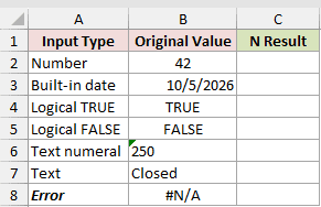
I want to see the numeric result for each original value.
Here is the formula in C2:
=N(B2)
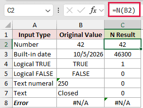
Fill the formula down through C8. N keeps 42 as 42, turns the built-in date into 46300, and converts TRUE to 1 and FALSE to 0.
The text numeral 250 is text, so N returns 0. The text Closed also returns 0, while the #N/A error stays #N/A.
Example 2: Return Date Serial Numbers
Here is a practical use for a date conversion.
Below is a milestone schedule with dates in the Scheduled Date column.
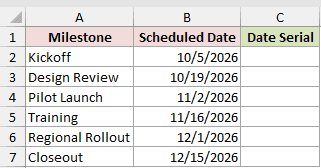
I want to expose the serial number behind each scheduled date.
Here is the formula in C2:
=N(B2)
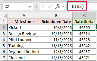
Fill the formula down through C7. The October 5, 2026 date returns 46300, and the later dates return their own serial values.
Use this when another system needs the serial value. It does not change how a date is formatted for display.
Example 3: Add a Note to a Numeric Formula
N can add a text note to a numeric formula because text passed to N returns zero.
Below is a small planning card with planned units, unit cost, and projected spend.
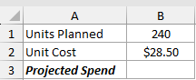
I want to keep a short planning note inside the projected-spend calculation.
Here is the formula:
=B1*B2+N("Approved Q3 planning assumption")
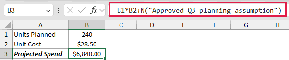
B1*B2 calculates 240 units at $28.50 each. N turns the text note into zero, so the result remains $6,840.00.
Pro Tip: This technique only works when the main formula returns a number. Use a cell comment or Note when the explanation needs to be visible without opening the formula.
Example 4: Coerce a Boolean Test in SUMPRODUCT
N can also turn a TRUE/FALSE test into 1s and 0s for arithmetic.
Below is a credit-request table with decisions and credit amounts.
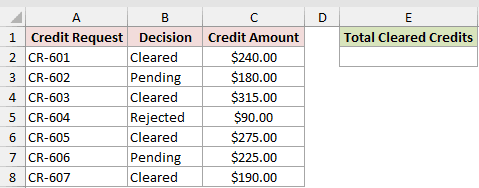
I want to total the credit amounts for cleared requests only.
Here is the formula:
=SUMPRODUCT(N(B2:B8="Cleared"),C2:C8)
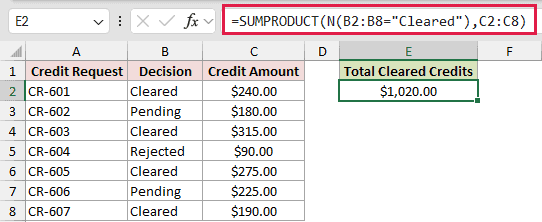
The comparison returns TRUE for the four cleared rows. N converts those TRUE values to 1 and the other results to 0.
SUMPRODUCT multiplies those 1s and 0s by the credit amounts. The total is $1,020.00.
For this single condition, SUMIFS is usually easier to read. This example shows how N helps inside an array calculation.
Tips & Common Mistakes
- N is not a text-to-number converter.
=N("250")returns 0, so use VALUE when you need 250. - N returns 1 for TRUE and 0 for FALSE.
- A built-in Excel date returns its serial number. That serial can vary if a workbook uses a different date system.
- N leaves error values as errors. It does not repair or hide them.
- Excel usually converts values automatically. N is mainly a compatibility function, with a few useful formula techniques.
N is most useful when you need its specific conversion rules inside a formula. I hope you found this article helpful.
Other Excel articles you may also like:
