
The ISODD function in Excel checks a number and returns TRUE when it is odd or FALSE when it is even.
It works with stored values, calculated totals, and record numbers. ISODD truncates decimals before testing them, so 2.9 is treated as 2.
In this article, I’ll show you how to identify odd numbers, assign packing lanes, and filter or count odd-numbered records.
ISODD Function Syntax in Excel
The ISODD function needs one argument:
=ISODD(number)
numberis the value, cell reference, or numeric range you want to test. Excel truncates nonintegers before testing them.
When to Use ISODD Function
- Flag odd-numbered IDs, jobs, tickets, or transactions.
- Assign alternating categories based on odd and even numbers.
- Return or count records whose identifying numbers are odd.
- Check whether a calculated total is odd before taking another action.
Example 1: Check Odd Numbers in a List
I’ll start with a list of service job numbers.
Below is the dataset with eight job numbers and an empty result column for the parity test.
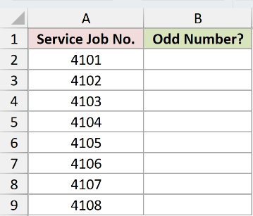
I want Excel to identify every odd-numbered service job with one formula.
Here is the formula:
=ISODD(+A2:A9)
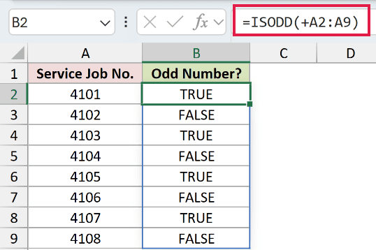
The unary plus before A2:A9 passes the range as numeric values. ISODD then returns TRUE for 4101, 4103, 4105, and 4107.
The single formula spills eight results from B2 through B9 in Excel 2021, Excel 2024, Microsoft 365, and Excel for the web.
Pro Tip: Keep the cells below the formula empty. Any obstruction in the intended output range causes a #SPILL! error.
Example 2: Assign Packing Lanes With ISODD
A TRUE or FALSE result can also drive a useful label.
Below is a packing list with batch numbers, products, and an empty Packing Lane column.
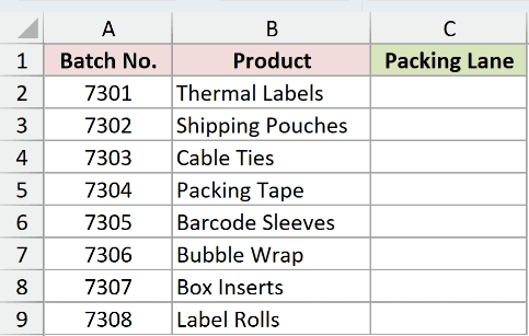
I want odd batches assigned to Lane A and even batches assigned to Lane B.
Here is the formula:
=IF(ISODD(+A2:A9),"Lane A","Lane B")
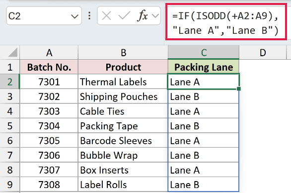
ISODD creates an array of TRUE and FALSE values from the batch numbers. The IF function returns the corresponding lane for each result.
Batch 7301 goes to Lane A, while batch 7302 goes to Lane B. The pattern continues through the list.
Pro Tip: Use ISEVEN when the rule is easier to express from the even side. For this example, ISODD keeps the Lane A test direct.
Example 3: Filter Odd-Numbered Records
ISODD can also act as a condition inside another formula.
Below is a return log and an empty output area with matching headers on the right.
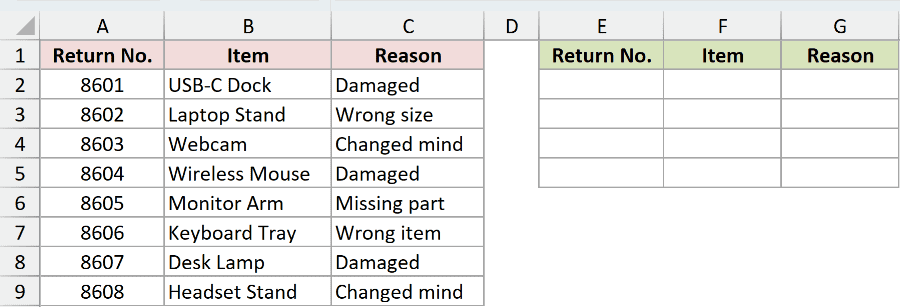
I want a separate list containing only returns with odd record numbers.
Here is the formula:
=FILTER(A2:C9,ISODD(+A2:A9))
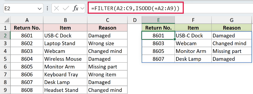
ISODD tests the Return No. column and creates the include array for the FILTER function.
FILTER returns the complete rows for returns 8601, 8603, 8605, and 8607. Their item and reason values come across with them.
Pro Tip: FILTER is available in Excel 2021, Excel 2024, Microsoft 365, and Excel for the web. Older versions can use an ISODD helper column and a regular filter.
Example 4: Count Odd Values With ISODD
Sometimes you need one count instead of a TRUE or FALSE result for every row.
Below is a list of 11 quality ticket numbers with a count card beneath it.
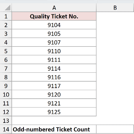
I want to count how many quality tickets have odd numbers.
Here is the formula:
=SUMPRODUCT(--ISODD(+A2:A12))
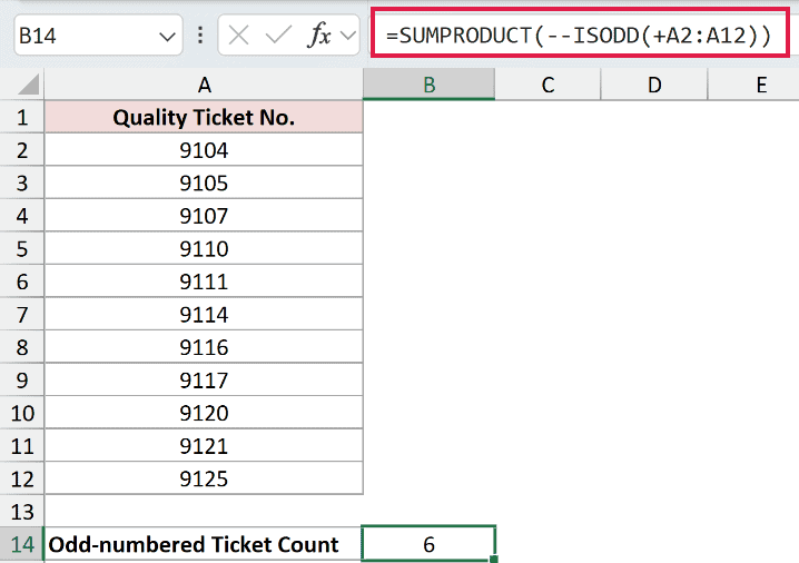
ISODD returns TRUE for six ticket numbers. The double unary changes TRUE to 1 and FALSE to 0, then SUMPRODUCT adds the results.
The final count in B14 is 6.
Example 5: Test Calculated Totals for Oddness
The number tested by ISODD can come from another formula.
Below are three carton counts for each shipment, plus empty Total Pieces and Odd Total columns.
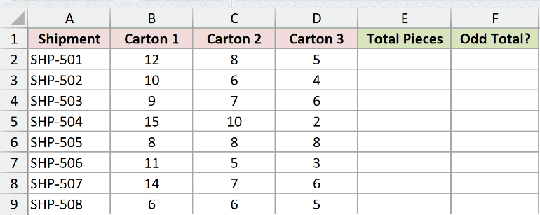
I first want to calculate each shipment total.
Here is the totaling formula:
=B2:B9+C2:C9+D2:D9
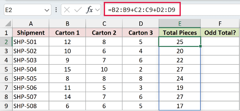
Excel adds the three carton columns row by row and spills the totals into E2:E9. The first shipment has 25 pieces.
Next, I want to test every spilled total for oddness.
Here is the ISODD formula:
=ISODD(+E2#)
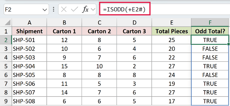
The spill operator in E2# refers to the complete array produced from E2. Unary plus passes those spilled totals to ISODD as numeric values.
ISODD returns TRUE for totals 25, 27, 19, 27, and 17. It returns FALSE for 20, 22, and 24.
Pro Tip: A spilled range reference such as E2# expands or contracts with its source formula, so the ISODD results stay aligned.
Example 6: Decimals, Negatives, and Text
ISODD behaves differently with decimals, negative numbers, and text.
Below is a short input list containing all three types and an empty result column.
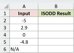
I want to see exactly how ISODD handles each input.
Here is the formula:
=ISODD(+A2:A6)
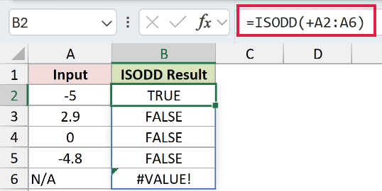
Negative integers work normally, so -5 returns TRUE. Excel truncates decimals toward zero before testing them, making 2.9 and -4.8 even.
Zero is even, so it returns FALSE. The text value N/A cannot be tested as a number and returns #VALUE!.
Tips & Common Mistakes
- ISODD returns TRUE or FALSE. Nest it inside IF when you need labels or actions instead.
- Decimal values are truncated before the test. ISODD tests 5.9 as 5 and -4.8 as -4.
- Nonnumeric input returns
#VALUE!. Clean or validate mixed data before testing it. - Keep spill ranges clear in Excel 2021 and later. A blocked output cell causes
#SPILL!. - In Excel 2019 and earlier, enter a single-cell formula and copy it down instead of using a spilling range formula.
- Use MOD when you need the remainder itself. Use ISODD when you only need a direct odd-or-even test.
I covered direct tests, labels, filtered records, counts, calculated totals, and the input behavior that can otherwise cause surprises.
I hope you found this article helpful.
Related Excel Functions / Articles:
Other Excel articles you may also like:
