
The PERCENTRANK.EXC function in Excel returns a value’s relative position within a dataset using an exclusive percentile rank.
You can use it to see where a sales total, listing price, or completion time sits among comparable values. Higher values receive higher ranks.
The exclusive method places the sample’s endpoints inside the percentage scale.
In this article, I’ll show you how to rank a list, handle values between or outside your data, and convert an exclusive rank back into a value.
PERCENTRANK.EXC Function Syntax in Excel
PERCENTRANK.EXC takes a comparison dataset, the value to rank, and an optional precision setting:
=PERCENTRANK.EXC(array, x, [significance])
- array (required) is the numeric dataset you’re ranking against.
- x (required) is the value whose relative position you want. A value between existing data points can be ranked through interpolation.
- significance (optional) sets how many decimal places Excel keeps. When omitted, Excel keeps three decimal places. It truncates the result rather than rounding it.
PERCENTRANK.EXC is available in Excel 2010 and later.
When to Use PERCENTRANK.EXC Function
- Rank sales totals against the same comparison group using the exclusive convention.
- Find where a proposed price sits between existing prices.
- Compare new measurements against a historical dataset and identify values outside its range.
- Keep percentile ranks consistent with calculations that also use the exclusive method.
Example 1: Rank Every Agent’s Sales
Let’s start with a list where each agent is ranked against the whole team.
Below is the dataset. Column A lists agents, column B contains homes sold, and column C will show each agent’s percent rank.
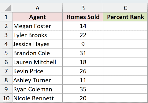
We want to calculate an exclusive percentile rank for every sales total without rearranging the list.
Enter this formula in C2:
=PERCENTRANK.EXC($B$2:$B$10,B2:B10)
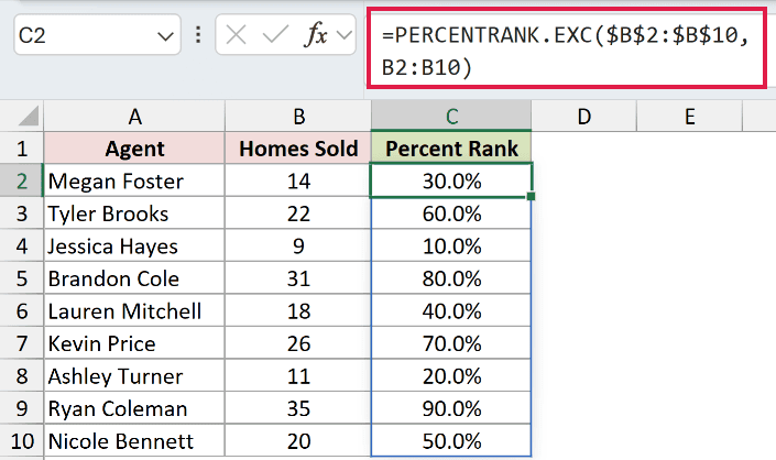
The absolute reference $B$2:$B$10 identifies the comparison group. The second range, B2:B10, asks Excel to rank every sales total against it.
The results spill from C2 through C10 in Excel 2021, Excel 2024, and Microsoft 365. Enter the formula only in C2.
In Excel 2019 and earlier, use a single sales cell for x and copy that per-row formula down, keeping the comparison range fixed.
For distinct values, the exclusive method uses the ascending position divided by the number of values in the list plus one. Your source rows don’t need sorting.
Megan Foster’s 14 homes sold returns 30.0%. Jessica Hayes has the lowest total, 9, and returns 10.0%.
Ryan Coleman’s 35 homes sold returns 90.0%. Being the largest observed value doesn’t put him at the top endpoint of the percentage scale.
The percentages describe relative position within this list. They aren’t each agent’s share of total homes sold.
Example 2: Compare Inclusive and Exclusive Ranks
Now let’s see how the ranking convention changes the same dataset.
Below is the dataset. Columns A and B hold gym locations and weekly check-ins. Columns C and D will contain inclusive and exclusive ranks.
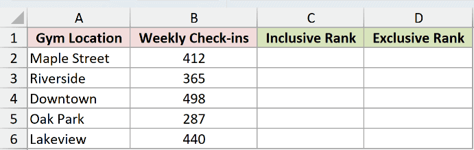
We want to compare every location’s exclusive rank with its inclusive rank.
For the comparison, PERCENTRANK.INC ranks values on a scale that includes the endpoints. Enter its formula in C2:
=PERCENTRANK.INC($B$2:$B$6,B2:B6)
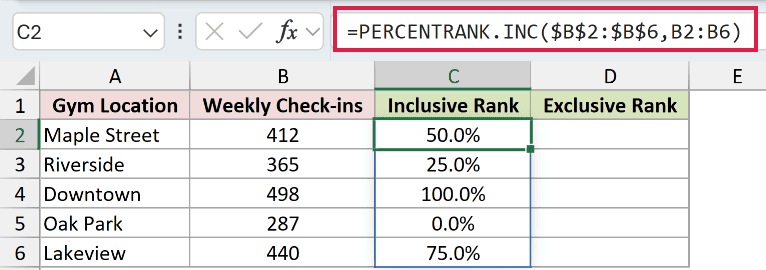
The comparison spills through C6. Oak Park’s 287 check-ins returns 0.0%, while Downtown’s 498 returns 100.0%.
Next, enter the PERCENTRANK.EXC formula in D2:
=PERCENTRANK.EXC($B$2:$B$6,B2:B6)
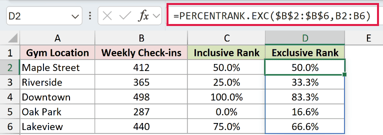
The exclusive results spill through D6. Oak Park now shows 16.6%, and Downtown shows 83.3%.
The difference also affects values inside the range. Riverside moves from 25.0% to 33.3%, while Lakeview moves from 75.0% to 66.6%.
The default three-digit precision truncates the ranks, which is why you see 16.6% and 66.6%.
Maple Street returns 50.0% with both methods. Changing the convention changes the spacing of the ranks, while the locations retain their relative order.
Keep the ranking convention consistent across reports you intend to compare.
Example 3: Rank a Price Between Listings
A value doesn’t have to appear in your dataset to receive a rank.
Below is the dataset. Columns A and B list used cars and asking prices. D2 holds your proposed price, with result cells in E2 and F2.
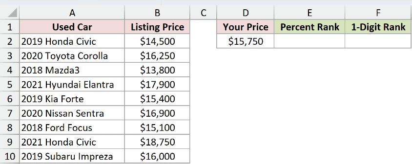
We want to rank the proposed price against the listings, then see how reduced precision affects that rank.
Enter the default-precision formula in E2:
=PERCENTRANK.EXC($B$2:$B$10,D2)
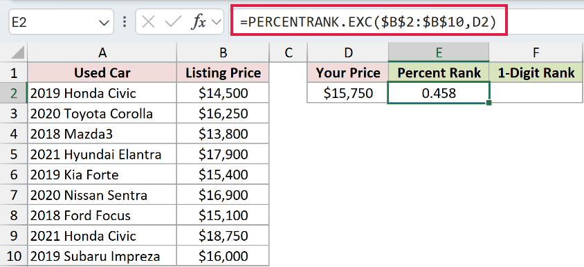
The proposed $15,750 price returns 0.458. This cell displays a decimal rank, rather than a percentage.
That price falls between $15,400 and $16,000. Excel interpolates, placing its rank proportionally between the ranks of those neighboring prices.
You don’t need to add your proposed price to the comparison list. Doing so would change the dataset you’re ranking against.
To keep fewer digits, enter this formula in F2:
=PERCENTRANK.EXC($B$2:$B$10,D2,1)
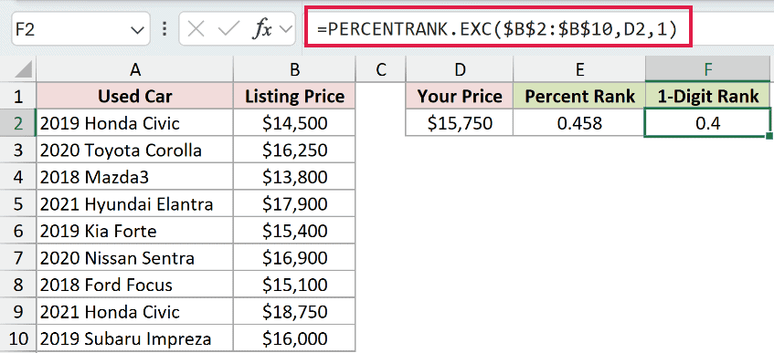
F2 returns 0.4. The significance argument discards later digits; it doesn’t round the rank to the nearest displayed decimal.
Pro Tip: If you only want a shorter display, change the cell’s number format. Changing significance changes the result available to later calculations.
Example 4: Handle Values Outside the Dataset
New measurements can fall beyond anything in your historical list.
Below is the dataset. Columns A and B contain historical newsletter sign-ups. D2:D5 holds new weekly totals, and columns E and F will show their ranks.
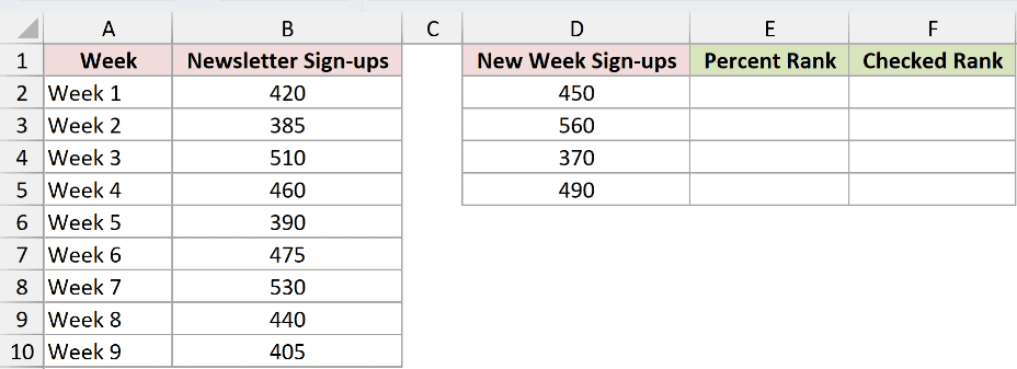
We want to rank new weekly totals against history and label the ones outside the historical range.
Enter this formula in E2:
=PERCENTRANK.EXC($B$2:$B$10,D2:D5)
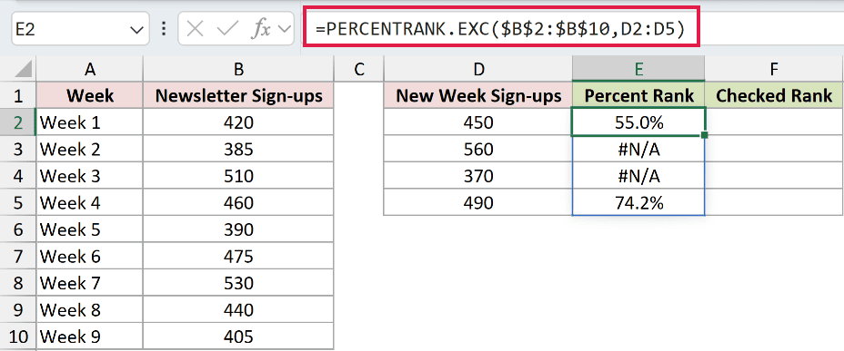
The formula spills through E5. The new totals 450 and 490 return 55.0% and 74.2%, respectively.
The #N/A results in E3 and E4 appear on purpose. The new total 560 exceeds the historical maximum, 530; the new total 370 falls below the minimum, 385.
PERCENTRANK.EXC interpolates inside the observed range. It doesn’t extend that range to assign a rank to a new high or low.
IFERROR replaces a formula’s error with a message. Here, it lets us label the out-of-range PERCENTRANK.EXC results while keeping valid ranks.
Enter the checked formula in F2:
=IFERROR(PERCENTRANK.EXC($B$2:$B$10,D2:D5),"Out of range")
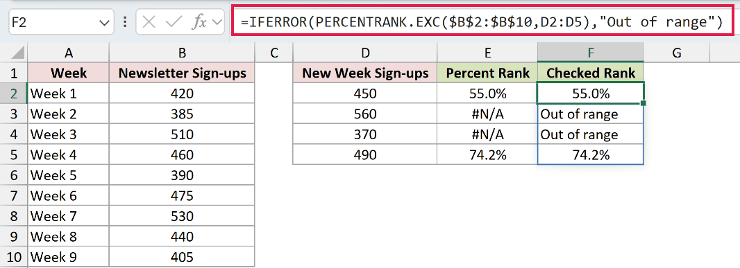
F3 and F4 now display Out of range. F2 and F5 still show 55.0% and 74.2%.
Pro Tip: IFERROR catches every error, so this label is appropriate only after checking your inputs. An empty comparison range or invalid argument could otherwise receive the same misleading message.
Example 5: Convert an Exclusive Rank Back
Keep the exclusive convention when you need to recover the value behind a rank.
Below is the dataset. Columns A and B contain orders and preparation times. D2 holds a target time, and E2:G2 will show the rank and conversion checks.
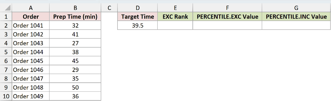
We want to rank the target preparation time, recover it from that rank, and demonstrate what happens when the conventions don’t match.
First, enter the PERCENTRANK.EXC formula in E2:
=PERCENTRANK.EXC($B$2:$B$10,D2)
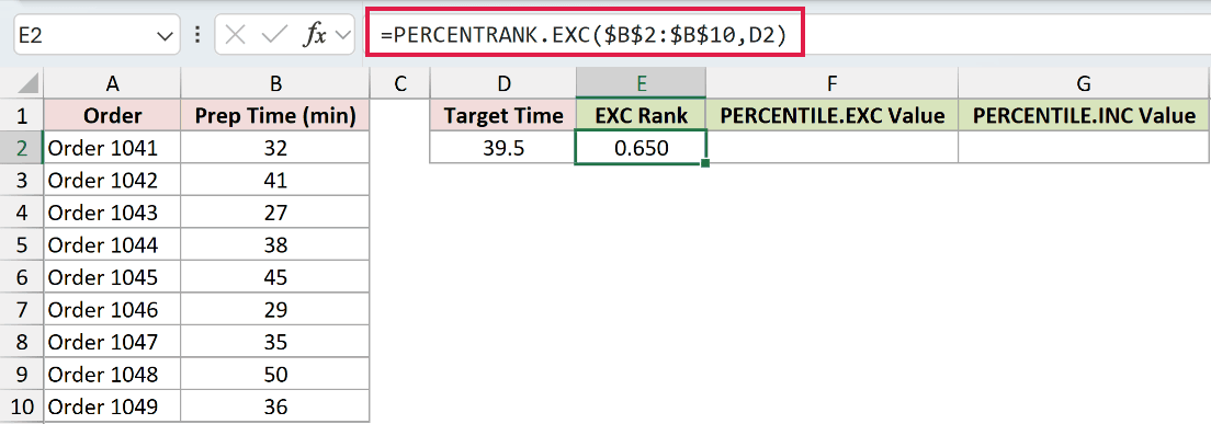
The target time of 39.5 minutes returns 0.650.
PERCENTILE.EXC works in the reverse direction: it takes an exclusive percentile rank and returns the corresponding dataset value. That makes it the matching choice for this check.
Enter this formula in F2:
=PERCENTILE.EXC($B$2:$B$10,E2)
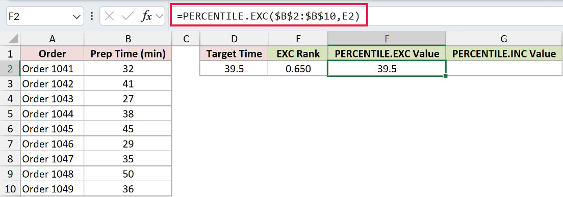
F2 returns 39.5, matching the original target time. Both calculations use the same data and the exclusive convention.
PERCENTILE.INC also converts a percentile rank into a value, but uses the inclusive convention. This mismatched convention changes the value recovered from PERCENTRANK.EXC.
Enter that comparison in G2:
=PERCENTILE.INC($B$2:$B$10,E2)
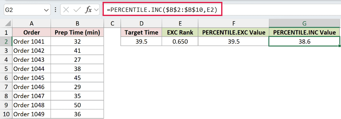
The mismatched comparison returns 38.6. Excel hasn’t reported an error, but the result no longer matches the target.
Pro Tip: This example recovers the target exactly. Don’t assume every conversion will: PERCENTRANK.EXC can truncate the rank before the matching percentile calculation receives it.
Tips & Common Mistakes
- Check the comparison range before hiding errors. In testing, an empty array returned
#N/A, as did a value outside the dataset’s minimum and maximum. - Check significance and input types. A significance argument of 0 returned
#NUM!; nonnumeric text supplied asxreturned#VALUE!in testing. - Ties share the lowest occupied position. Equal values receive the same exclusive rank, rather than an average of their occupied positions.
- Distinguish size from performance. A higher rank means a larger input. For preparation times, a higher rank means a longer wait, which may be worse.
- Keep the comparison group consistent. Changing which observations belong to the dataset changes what the resulting rank means.
Related Excel Functions / Articles:
