PERCENTILE.EXC Function in Excel

The PERCENTILE.EXC function in Excel returns an exclusive percentile from a set of numeric values.

PERCENTILE.EXC rejects k values of 0 and 1, plus values too close to either end for the sample size. Small datasets can therefore return #NUM! for a valid-looking k.

In this article, I’ll show you how to find the valid k range, compare exclusive and inclusive results, and calculate separate cutoffs for groups.

PERCENTILE.EXC Function Syntax in Excel

The PERCENTILE.EXC function uses a data array and a percentile value.

=PERCENTILE.EXC(array, k)

• array (required) is the range or array containing the numeric data.
• k (required) identifies the exclusive percentile. Enter it as a decimal or percentage greater than 0 and less than 1. For n numeric values in array, usable k runs from 1/(n+1) to n/(n+1).

When to Use PERCENTILE.EXC Function

• Follow an analysis method that specifically requires exclusive percentiles.
• Check whether a percentile is valid for the size of a sample.
• Compare exclusive and inclusive percentile thresholds.
• Calculate exclusive quartiles and the interquartile range.
• Set separate percentile cutoffs for categories or review flags.

Example 1: Calculate an Exclusive Percentile

Let’s start with a straightforward supplier analysis.

Below is the dataset. Columns A and B contain vendors and lead times, while the labeled cell in column D will hold the 90th percentile.

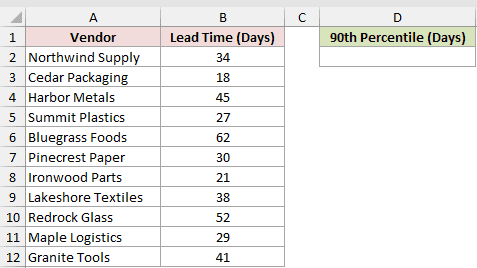
We want to find the exclusive 90th percentile of the lead times.

Here is the formula:

=PERCENTILE.EXC(B2:B12,0.9)

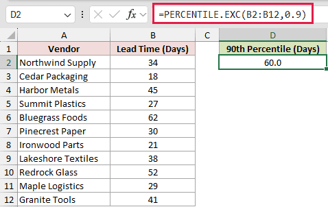
The formula returns 60.0 days. Excel orders the values internally and interpolates because the requested percentile falls between two observations.

The 60.0 result is not one of the lead times in column B.

Example 2: Find the Valid k Range

Small samples make the valid k range especially important.

Below is the dataset. Webinar registrations are in columns A and B, k values are in D, and the empty Registrations at k column is in E.

Columns G and H contain the labeled Smallest Valid k and Largest Valid k cells.

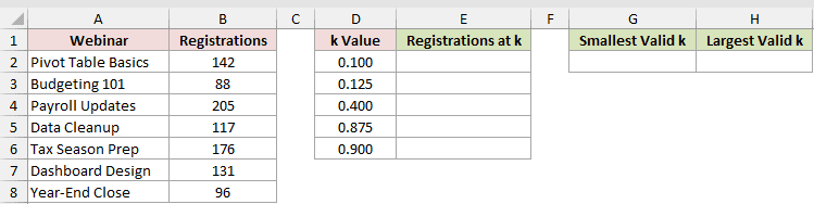
We want to calculate the smallest and largest valid k values, then test every k in column D.

Here is the formula for the smallest valid k:

=1/(COUNT(B2:B8)+1)

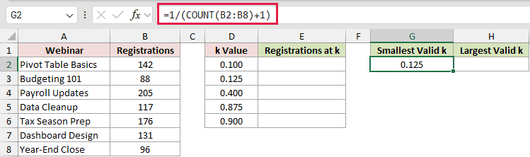
The formula returns 0.125.

Here is the formula for the largest valid k:

=COUNT(B2:B8)/(COUNT(B2:B8)+1)

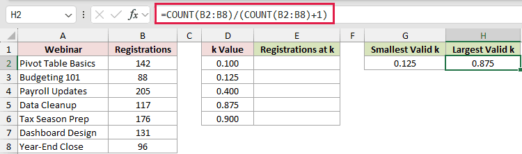
This formula returns 0.875.

These boundaries equal 1/(n+1) and n/(n+1) for the 7 numeric registrations in B2:B8.

Now use those boundaries to interpret the k list:

=PERCENTILE.EXC($B$2:$B$8,D2:D6)

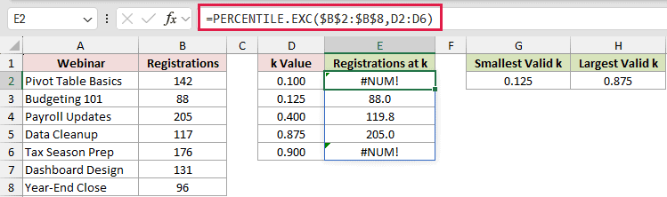
The single formula spills results beside the k values. Range formulas that spill need Excel 2021, Excel 2024, or Microsoft 365.

The exact boundary values return 88.0 and 205.0, which are the minimum and maximum registrations.

The 0.100 and 0.900 inputs fall outside the Smallest Valid k and Largest Valid k boundaries, so E2 and E6 deliberately return #NUM!.

Pro Tip: Count numeric observations, not rows, when checking the valid range. Blank cells, text, and logical values in a referenced array do not increase the numeric count.

Example 3: Compare PERCENTILE.EXC and PERCENTILE.INC

Now let’s see how the exclusive and inclusive methods differ.

Below is the dataset. It lists listing IDs, days on market, and k values, with separate result columns for PERCENTILE.EXC and PERCENTILE.INC.

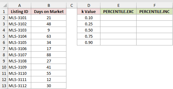
We want both percentile methods calculated across the same five k values.

Here is the exclusive formula:

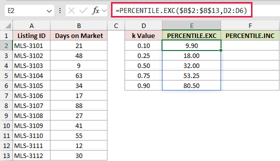
=PERCENTILE.EXC($B$2:$B$13,D2:D6)

And here is the inclusive formula:

=PERCENTILE.INC($B$2:$B$13,D2:D6)

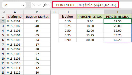
Both formulas spill down their result columns. At k = 0.50, both return 32.00 days.

The difference appears toward the tails. At 0.10, EXC returns 9.90 while INC returns 12.50. At 0.90, the results are 80.50 and 62.20.

The older PERCENTILE function follows the inclusive method, so it matches PERCENTILE.INC rather than PERCENTILE.EXC.

Example 4: Calculate Exclusive Quartiles and IQR

PERCENTILE.EXC can also calculate exclusive quartiles and the interquartile range.

Below is the dataset. It contains household electric bills and a calculation panel with labeled result cells for both quartiles and the interquartile range.

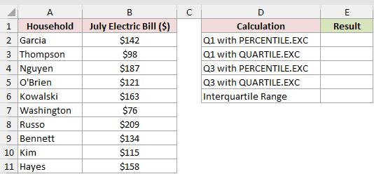
We want to calculate each exclusive quartile two ways, then subtract the lower quartile from the upper quartile.

Here is the PERCENTILE.EXC formula for Q1:

=PERCENTILE.EXC($B$2:$B$11,0.25)

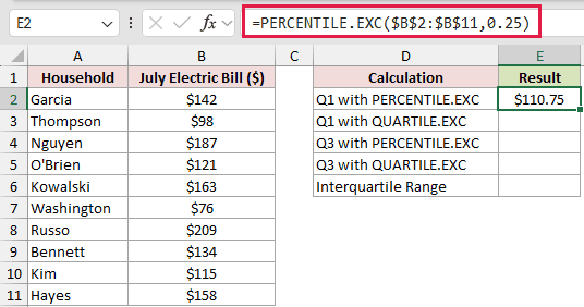
It returns $110.75.

Here is the equivalent QUARTILE.EXC formula:

=QUARTILE.EXC($B$2:$B$11,1)

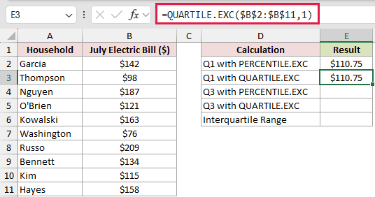
QUARTILE.EXC also returns $110.75 for Q1.

Here is the PERCENTILE.EXC formula for Q3:

=PERCENTILE.EXC($B$2:$B$11,0.75)

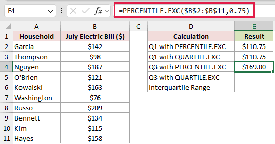
It returns $169.00.

Here is the matching QUARTILE.EXC formula:

=QUARTILE.EXC($B$2:$B$11,3)

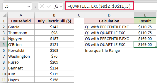
This formula also returns $169.00 for Q3.

Finally, subtract the exclusive lower quartile from the upper quartile:

=PERCENTILE.EXC($B$2:$B$11,0.75)-PERCENTILE.EXC($B$2:$B$11,0.25)

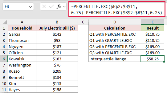
The exclusive interquartile range is $58.25. The inclusive method returns $45.25 for the same bill data, so the chosen percentile convention changes the spread.

Example 5: Calculate Percentiles by Category

Here’s a practical way to calculate separate cutoffs for different groups.

Below is the dataset. It lists jobs, service types, and job lengths, plus a summary table for counts and two percentile results.

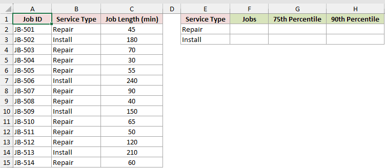
We want to count each service type before calculating its 75th and 90th percentiles.

First, count the jobs for the service type in E2:

=COUNTIF($B$2:$B$15,$E2)

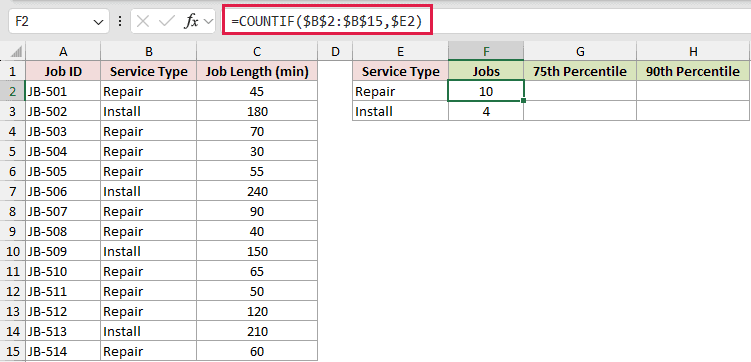
Copy the formula down through F3. It returns 10 repair jobs and 4 install jobs.

Next, calculate the 75th percentile for each filtered group. The FILTER function needs Excel 2021 or later.

=PERCENTILE.EXC(FILTER($C$2:$C$15,$B$2:$B$15=$E2),0.75)

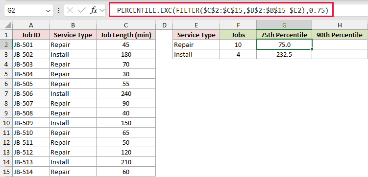
Copy this formula through G3. It returns 75.0 minutes for repairs and 232.5 minutes for installations.

Now calculate the 90th percentile:

=PERCENTILE.EXC(FILTER($C$2:$C$15,$B$2:$B$15=$E2),0.9)

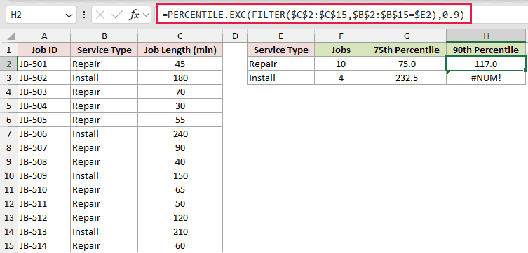
Copy the formula through H3. Repairs return 117.0 minutes, while the installation result deliberately returns #NUM!.

The install group contains 4 jobs, so its 0.9 input falls outside that group’s valid exclusive range. PERCENTILE.INC would return 231.0 instead.

Pro Tip: Count each filtered group before requesting an extreme percentile. A k value that works for a larger group may return #NUM! for a smaller one.

Example 6: Flag Values Above a Percentile

Finally, let’s turn an exclusive percentile into a review rule.

Below is the dataset. It contains claim IDs, employee names, and amounts, with a result column ready to hold each review flag.

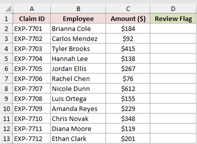
We want to label every claim above the 80th percentile as Review and every other claim as OK.

Here is the formula:

=IF(C2:C13>PERCENTILE.EXC(C2:C13,0.8),"Review","OK")

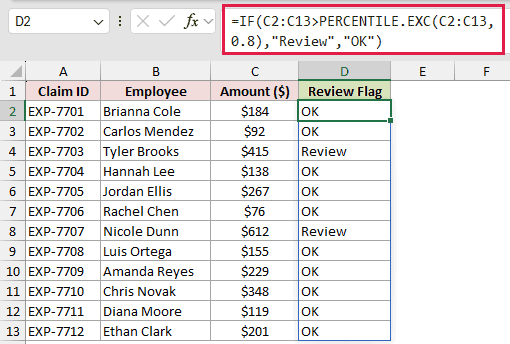
The percentile cutoff is 374.8. The comparison runs across the amount range, so one formula spills all the flags into column D.

Tyler Brooks’s $415 claim and Nicole Dunn’s $612 claim return Review. Every other claim returns OK.

Tips & Common Mistakes

• A k value entered as 40% works the same way as its decimal equivalent.
• Text entered for k returns #VALUE!, while an empty numeric array returns #NUM!.
• The valid k range depends on the count of numeric values. The lower edge returns the minimum, and the upper edge returns the maximum. A k just outside either edge returns #NUM!.
• PERCENTILE.EXC returns one result for one k. Give it a range of k values when you want a spilled list of percentile results.
• Keep the spill area empty. A non-empty cell in the spill range makes the formula return #SPILL!.
• QUARTILE.EXC at quart 0 returns #NUM! because the exclusive method does not include that endpoint.
• Use PERCENTILE.INC when your method needs the inclusive endpoints. The legacy PERCENTILE function also follows the inclusive calculation.

I showed you how the valid k window limits exclusive percentiles and why EXC and INC differ most near the tails.

We also used PERCENTILE.EXC for quartiles, group-specific cutoffs, and review flags.

List of All Excel Functions

Related Excel Functions / Articles:

• QUARTILE.INC Function in Excel
• PERCENTRANK.INC Function in Excel
• How to Find Percentile in Excel (PERCENTILE Function)