
Excel’s RANDARRAY function returns an array of random numbers with the row count, column count, limits, and number type you choose.
One formula can fill a block with whole numbers or decimals. The values change whenever Excel recalculates, so copy and paste values when you need to keep a draw.
In this article, I’ll show you how to generate grids of random numbers, choose numeric bounds, and pick random items from a list.
RANDARRAY Function Syntax in Excel
The RANDARRAY function can generate one random value or a grid of random values.
=RANDARRAY([rows],[columns],[min],[max],[whole_number])
- rows (optional) is the number of rows to return. It defaults to 1.
- columns (optional) is the number of columns to return. It defaults to 1.
- min (optional) is the lowest possible number. It defaults to 0.
- max (optional) is the upper limit for the random numbers. It defaults to 1.
- whole_number (optional) is TRUE for whole numbers or FALSE for decimals. It defaults to FALSE.
When to Use RANDARRAY Function
- Fill a multirow, multicolumn range with random numbers from one formula.
- Generate whole numbers or decimals within limits you choose.
- Create sample data for testing formulas, reports, and worksheet layouts.
- Select several random items from a list when repeated picks are acceptable.
- Feed many random trials directly into another function without displaying the full array.
Example 1: Generate a Grid of Whole Numbers
Let’s start with the kind of task RANDARRAY handles best.
Below is the dataset. Column A lists eight days.
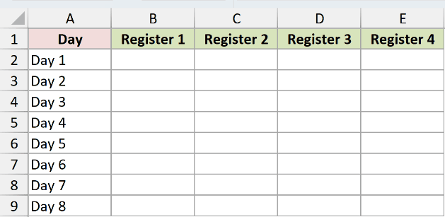
We want one formula to generate an 8-row by 4-column grid of whole-number transaction counts from 20 to 120.
Here is the formula:
=RANDARRAY(8,4,20,120,TRUE)
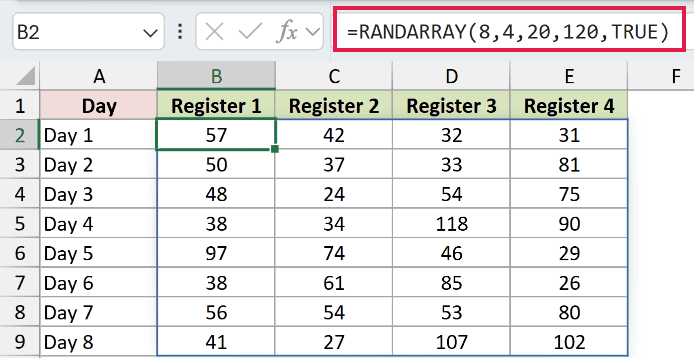
The first two arguments set the output to eight rows and four columns. The next two set the lower and upper limits.
TRUE tells Excel to return whole numbers. Every cell in B2:E9 contains a whole number from 20 to 120, and repeats are normal.
The formula in B2 alone fills the entire 32-cell area.
Pro Tip: Keep B2:E9 empty before entering the formula. Any existing content inside the intended spill area causes a #SPILL! error.
Example 2: Return Decimals or Whole Numbers
Now let’s see what the final argument changes.
Below is the dataset. Column A labels eight random draws.
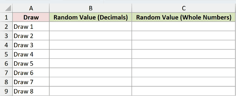
We want to compare random decimals with random whole numbers using the same limits.
Here is the formula with whole_number omitted:
=RANDARRAY(8,1,1,50)
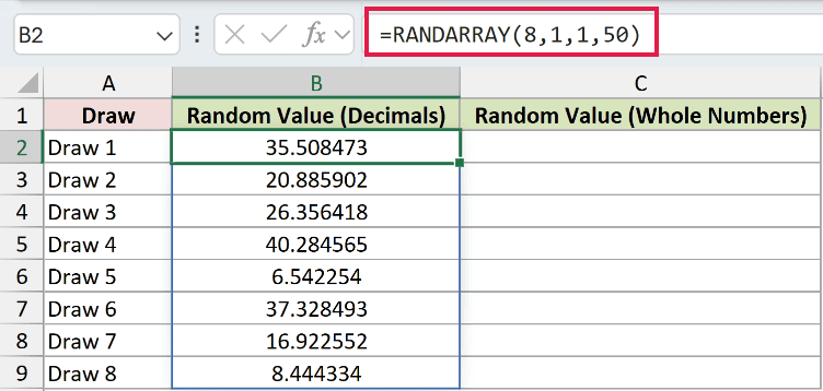
This formula spills eight decimals into B2:B9. Each decimal falls between 1 and 50 because whole_number defaults to FALSE.
Here is the formula that requests whole numbers:
=RANDARRAY(8,1,1,50,TRUE)
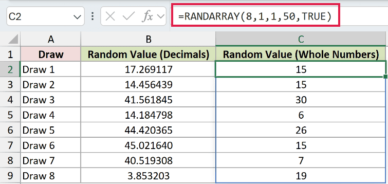
Adding TRUE changes the output type. The formula spills eight whole numbers from 1 to 50 into C2:C9, with both limits possible.
The whole_number argument replaces older RAND formulas that needed extra arithmetic or INT to produce values within chosen limits.
Example 3: Set Minimum and Maximum From Cells
Here’s a setup you can change without editing the formula.
Below is the dataset. Column A lists donors, empty column B awaits Sample Pledge, and D1:E3 contains the minimum and maximum pledge settings card.
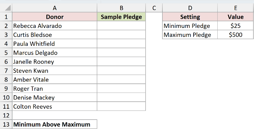
We want to generate ten sample pledges using the limits stored in the settings card.
Here is the formula:
=RANDARRAY(10,1,$E$2,$E$3,TRUE)
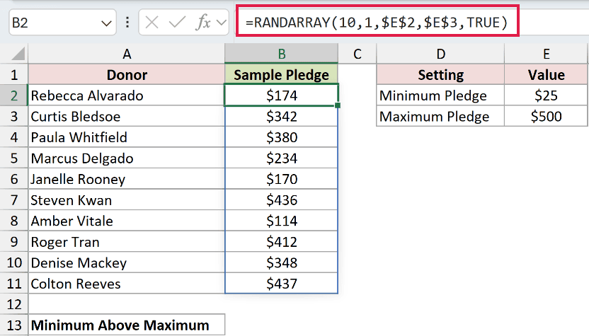
The formula spills ten whole-dollar amounts into B2:B11. Each amount falls between the minimum in E2 and the maximum in E3.
The absolute references keep both settings fixed. You can change either setting, and Excel generates a new set within the revised range.
In B13, beside the Minimum Above Maximum label, the next formula deliberately reverses the minimum and maximum to demonstrate what not to do:
=RANDARRAY(10,1,$E$3,$E$2,TRUE)
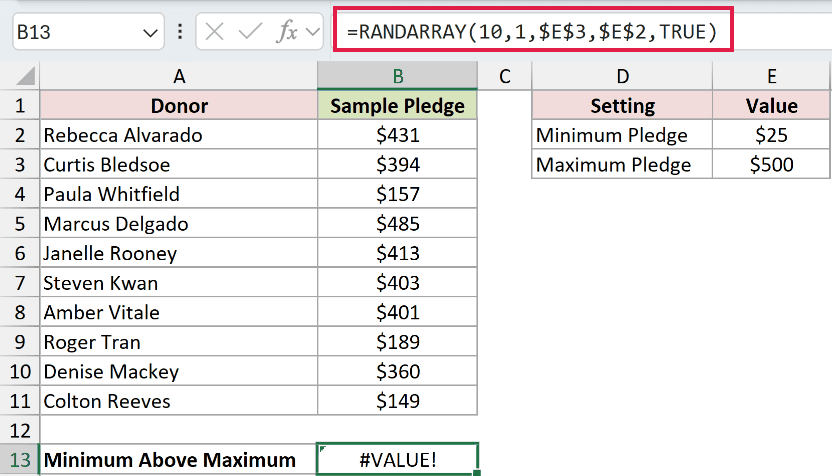
Because the minimum is greater than the maximum, B13 returns #VALUE!.
That bottom cell is a deliberate error demonstration, not an answer. B13 shows reversed limits rather than a valid pledge result.
Example 4: Pick Random Items From a List
RANDARRAY can also generate positions for another function to use.
Below is the dataset. Column A contains the available safety topics.
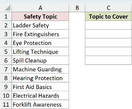
We want to draw five topics from the list with one spilling formula.
Here is the formula:
=INDEX($A$2:$A$11,RANDARRAY(5,1,1,COUNTA($A$2:$A$11),TRUE))
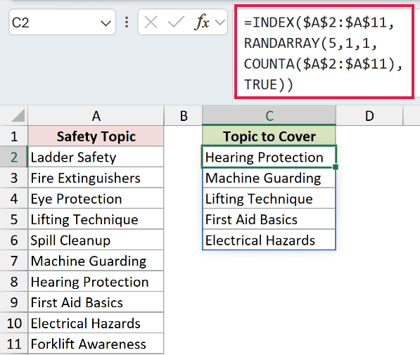
COUNTA finds the list length. RANDARRAY generates five whole-number positions, and INDEX returns the topic at each position into C2:C6.
Each position is generated independently, so the same topic can appear more than once. Use a no-duplicates approach when every pick must be unique.
Example 5: Return a Single Random Value
You do not have to create a large spill every time.
Below is a two-row card labeling a decimal draw and a whole-number draw.

We want to see how RANDARRAY behaves with no arguments and with a one-cell whole-number array.
Here is the formula with every argument omitted:
=RANDARRAY()
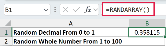
This returns one decimal between 0 and 1. It works like RAND for a single cell.
Here is the formula for one whole number:
=RANDARRAY(1,1,1,100,TRUE)
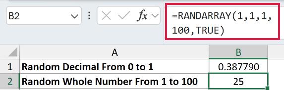
The two 1 arguments limit the array to one row and one column. The result is a whole number from 1 to 100.
This second formula does the same basic job as RANDBETWEEN. RANDARRAY becomes more useful when you increase its rows or columns.
Example 6: Use RANDARRAY Inside Another Function
Finally, the random array does not need to appear on the sheet.
Below is a two-row card labeling a dice-roll average and a coin-flip share.
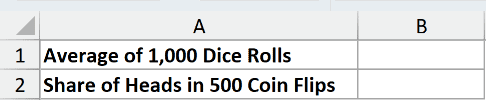
We want AVERAGE to summarize many random trials directly inside two cells.
Here is the formula for 1,000 dice rolls:
=AVERAGE(RANDARRAY(1000,1,1,6,TRUE))
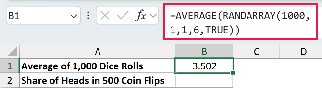
RANDARRAY generates 1,000 whole numbers from 1 to 6 in memory. AVERAGE reduces that array to one result close to 3.5.
Here is the formula for 500 coin flips:
=AVERAGE(RANDARRAY(500,1,0,1,TRUE))
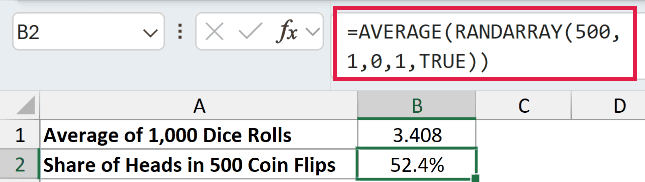
RANDARRAY treats 0 and 1 as the two possible outcomes. Their average is the share of 1s, which should stay close to 50% over many trials.
Pro Tip: To freeze random results, copy the cells and use Paste Special > Values. This replaces the formulas with their current values.
Tips & Common Mistakes
- RANDARRAY is volatile. Reopening the workbook, editing a cell, or pressing F9 can generate a fresh set of results.
- Omitting whole_number means FALSE, so Excel returns decimals. Add TRUE when you need whole numbers.
- Keep every cell in the intended output area empty. Otherwise, the formula returns #SPILL! because Excel cannot place the complete array.
- A spill reference such as
B2#refers to the entire array that begins in B2. Edit or clear the formula from its anchor cell. - Keep min less than or equal to max. Reversing them returns #VALUE!, not #NUM!.
- RANDARRAY is available in Microsoft 365, Excel 2021 and later, and Excel for the web. Excel 2019 and earlier return #NAME?.
- To freeze a single-cell RANDARRAY formula while editing it, select the formula in the formula bar and press F9 before confirming the entry.
RANDARRAY is most useful when you need many random values from one formula or want to pass those values straight into another calculation.
Set the size, limits, and number type first. Then freeze the results when you need a stable copy.
Related Excel Functions / Articles:
