
The RANDBETWEEN function in Excel returns a random integer between two limits, including both endpoints.
You can use it for sample data or random selections. Results change when the worksheet recalculates; paste them as values to keep a particular set.
For a whole grid of random numbers from one formula, RANDARRAY offers more control over the output size.
In this article, I’ll show you how to generate random dates and decimals, choose an item from a list, and create random multiples.
RANDBETWEEN Function Syntax in Excel
The RANDBETWEEN function uses a lower and upper limit to generate a random whole number.
=RANDBETWEEN(bottom, top)
- bottom (required) is the smallest whole number that Excel can return.
- top (required) is the largest whole number that Excel can return.
Both limits are included. For example, limits of 1 and 10 can return any whole number from 1 through 10.
When to Use RANDBETWEEN Function
- Create sample quantities, scores, IDs, or other whole-number test data.
- Generate random dates between two fixed dates.
- Create random decimal values by generating scaled integers and dividing them.
- Pick a random name, product, or other item from a list.
- Generate values that must follow fixed steps, such as multiples of 25.
Example 1: Generate Random Whole Numbers
Let’s start with a basic test-data example.
Below is the dataset. Column A contains eight test order IDs, and column B will hold an order quantity for each one.
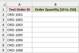
We want each order to receive a whole-number quantity from 10 to 250.
Enter this formula in B2 and copy it down through B9:
=RANDBETWEEN(10,250)
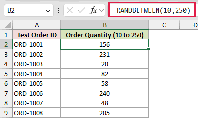
The formula can return any whole number from 10 through 250. Because both limits are included, 10 and 250 are possible results.
Each row calculates separately, so different orders can receive the same quantity.
Pro Tip: RANDBETWEEN is volatile. Its results can change after you edit the workbook, press F9, or reopen the file.
Example 2: Generate Random Dates in Excel
Now let’s create sample invoice dates for a reporting period.
Below is the dataset. Column A lists eight sample invoices, and column B will contain dates from the first quarter of 2026.
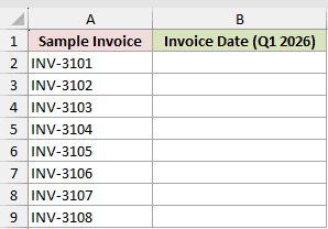
We want to assign each invoice a random date from January 1 through March 31, 2026.
The formula in B2, filled down through B9, is:
=RANDBETWEEN(DATE(2026,1,1),DATE(2026,3,31))
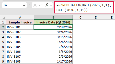
Excel stores dates as serial numbers. The two DATE functions supply the serial numbers for the first and last dates in the permitted range.
RANDBETWEEN returns a serial number between those limits, and the date format in column B displays it as a date.
Pro Tip: If the result appears as a five-digit number, apply a date format to the result cells. The formula itself does not add date formatting.
Example 3: Generate Random Decimal Numbers
RANDBETWEEN returns integers, but you can scale those integers to create decimal values.
Below is the dataset. Column A lists eight menu items, and column B will contain a sample price for each item.
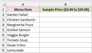
We want each sample price to fall between $4.99 and $29.99 in one-cent increments.
Here is the formula entered in B2 and copied down through B9:
=RANDBETWEEN(499,2999)/100
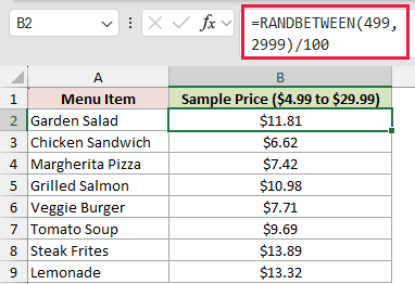
RANDBETWEEN first generates a whole number from 499 through 2999. Dividing that number by 100 converts it to a price from $4.99 through $29.99.
RANDBETWEEN only returns whole numbers, so the formula generates the cents first and divides the result by 100.
For a decimal from 0 up to, but not including, 1, use the RAND function.
In Excel 365 or Excel 2021 and later, RANDARRAY can return random decimals directly. RANDBETWEEN remains useful when you need exact scaled steps.
Example 4: Pick a Random Item From a List
Here’s how to use RANDBETWEEN inside another function.
Below is the dataset. Column A lists pull requests, column B will show the assignments, and D2:D7 contains the reviewer pool.
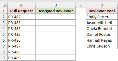
We want to assign one random reviewer from the six-name pool to each pull request.
Start with this formula in B2, then copy it down through B9:
=INDEX($D$2:$D$7,RANDBETWEEN(1,ROWS($D$2:$D$7)))
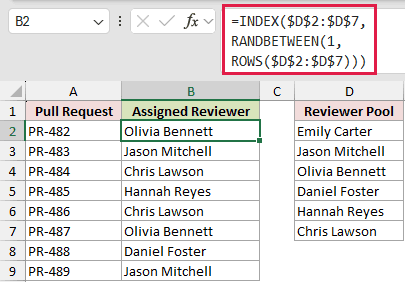
ROWS counts the six names in D2:D7. RANDBETWEEN then generates a position from 1 through 6, and INDEX returns the name at that position.
The absolute references keep the reviewer pool fixed as the formula is copied down.
Selections can repeat because each row makes an independent random pick. Use a shuffle-and-take approach when every person must be selected only once.
Example 5: Generate Random Multiples of 25
You can also limit random results to fixed intervals.
Below is the dataset. Column A lists eight employees, and column B will contain a spot bonus for each person.
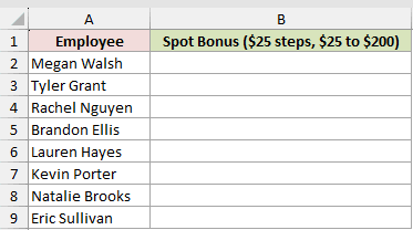
We want every bonus to be a multiple of $25, ranging from $25 through $200.
Here is the formula entered in B2 and copied down through B9:
=RANDBETWEEN(1,8)*25
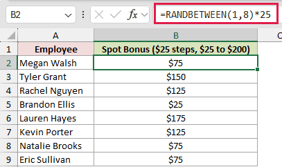
RANDBETWEEN generates a whole number from 1 through 8. Multiplying it by 25 limits the possible bonuses to $25 increments.
Change the multiplier to match another step size. For example, a multiplier of 10 would produce multiples of 10.
Example 6: RANDBETWEEN vs RANDARRAY
Finally, let’s compare the traditional formula with its dynamic array alternative.
Below is the dataset. Column A lists eight raffle tickets, while columns B and C will contain random draw numbers from the two functions.
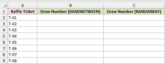
We want eight random whole numbers from 1 through 1000 using both approaches.
Here is the RANDBETWEEN formula entered in B2 and copied down through B9:
=RANDBETWEEN(1,1000)
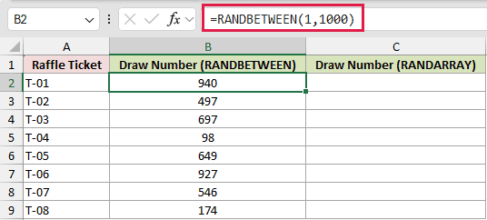
And here is the single RANDARRAY formula entered in C2:
=RANDARRAY(8,1,1,1000,TRUE)
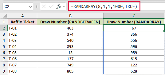
The RANDBETWEEN formula returns one number in each cell, so it must be copied down. Every cell can return a whole number from 1 through 1000.
RANDARRAY uses one formula to spill eight rows and one column. Its final TRUE argument tells Excel to return whole numbers rather than decimals.
Both functions are volatile, and either method can produce duplicate numbers.
Pro Tip: To keep generated results, copy the cells and use Paste Special > Values. This replaces the formulas with their current values.
Tips & Common Mistakes
- RANDBETWEEN includes both limits. A formula using 1 and 10 can return 1, 10, or any whole number between them.
- The function recalculates whenever Excel recalculates the workbook. Freeze finished results by copying them and pasting values.
- Make sure the bottom value is not greater than the top value. Otherwise, Excel returns a #NUM! error.
- Format random date results as dates. Without date formatting, Excel displays their underlying serial numbers.
- For decimals in fixed steps, use whole-number bounds that are 10 or 100 times larger, then divide the result, as in the price example.
- Use RANDARRAY in supported Excel versions when you want one formula to spill a block of random numbers.
RANDBETWEEN works well when you need one random whole number per formula, especially for quick sample data and random selections.
Once you have the set you want, copy it and paste values to stop the numbers from changing.
Related Excel Functions / Articles:
