How to Randomize a List in Excel

If you want to shuffle a list in Excel into a random order, you will notice there is no single “shuffle” button anywhere on the ribbon. That is because Excel treats sorting as an ordered operation, so it needs something random to sort by first.

The good news is that a couple of quick tricks handle this in seconds.

In this tutorial I’ll show you three ways to randomize a list: a one-formula method with RANDARRAY and SORTBY, a helper-column method with RAND, and a VBA macro for a repeatable one-click shuffle.

Method #1: Using RANDARRAY and SORTBY

If you are on Excel 365 or Excel 2021, this is the fastest way to randomize a list. A single dynamic-array formula shuffles the whole list at once and spills the result into a fresh range, leaving your original data untouched.

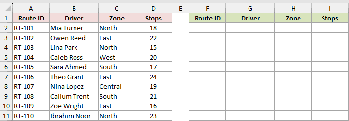
Below I have a list of delivery routes, with a Route ID, the assigned driver, the zone, and the number of stops. I want to reshuffle these rows into a random order.

Here is the formula:

=SORTBY(A2:D11,RANDARRAY(ROWS(A2:D11)))

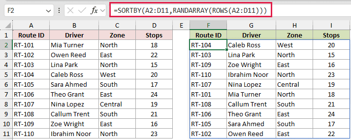
The formula spills down and across automatically, returning every original row in a new random order.

How does this formula work?

ROWS(A2:D11) counts how many rows are in the data, which is 10 here. RANDARRAY(10) then builds a column of 10 random decimals between 0 and 1.

SORTBY sorts the data range A2:D11 by that column of random numbers. Since the numbers are random, the rows come back in a random sequence. Every recalculation generates a fresh set of random numbers, so the list reshuffles each time.

Note: RANDARRAY is a volatile function, so the shuffle changes every time the sheet recalculates. To lock in one particular order, copy the spilled result and use Paste Special > Values to convert it to static values.

Method #2: Using the RAND Function

If you are on Excel 2019 or an older version, SORTBY is not available, so this is the method for you. You add a helper column of random numbers with the RAND function, then sort the list by that column.

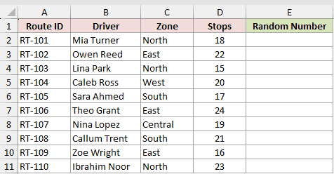
I’m using the same delivery routes list, with a Route ID, driver, zone, and stops. The goal again is to put these rows in a random order.

Here are the steps to randomize the list using RAND:

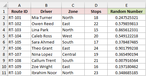
1. In cell E1, next to the last header, type Random Number to give the helper column a header. Then in E2, enter the formula =RAND().

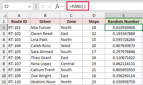
2. Copy the formula down to the last row of data, so E2:E11 all have a random number.

3. Click any single cell inside the data, including the helper column.

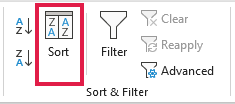
4. Go to the Data tab and click Sort.

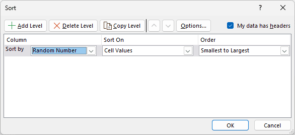
5. In the Sort dialog box, make sure My data has headers is checked, set Sort by to Random Number, and click OK.

The rows are now in a random order. Once you are happy with the shuffle, you can delete the helper column, since it has done its job.

Note: RAND generates new numbers whenever the sheet recalculates, which normally happens after an edit in Automatic calculation mode. That is fine here, because the sort already reordered your rows physically.

Method #3: Using VBA

If you shuffle lists often, a VBA macro lets you do it with one click or a keyboard shortcut. This one uses a Fisher-Yates shuffle, which is the standard way to give every row an equal chance of landing in any position.

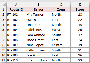
Here is the same delivery routes list I want to randomize.

Here is the VBA code:

Sub RandomizeList()
    Dim rng As Range
    Dim rowCount As Long, i As Long, j As Long
    Dim tempRow As Variant

    Set rng = Range("A2:D11")
    rowCount = rng.Rows.Count
    Randomize

    For i = rowCount To 2 Step -1
        j = Int(Rnd * i) + 1
        tempRow = rng.Rows(i).Value
        rng.Rows(i).Value = rng.Rows(j).Value
        rng.Rows(j).Value = tempRow
    Next i
End Sub

Sub RandomizeList()
    Dim rng As Range
    Dim rowCount As Long, i As Long, j As Long
    Dim tempRow As Variant

    Set rng = Range("A2:D11")
    rowCount = rng.Rows.Count
    Randomize

    For i = rowCount To 2 Step -1
        j = Int(Rnd * i) + 1
        tempRow = rng.Rows(i).Value
        rng.Rows(i).Value = rng.Rows(j).Value
        rng.Rows(j).Value = tempRow
    Next i
End Sub

Here are the steps to add and run this macro:

1. Press Alt + F11 to open the VBA editor, then go to Insert > Module.

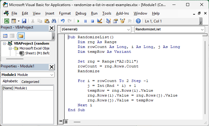
2. Paste the code above into the module window.

3. Click anywhere inside the code and press F5 to run it. Then switch back to your sheet.

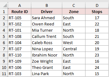
The rows in A2:D11 are now shuffled in place. Run the macro again any time you want a fresh order.

The code walks the list from the bottom row up. For each row i, it picks a random row j anywhere from row 1 up to and including row i itself (so a row can keep its spot), and swaps the values across A:D in those two rows. Randomize seeds the generator so you get a different shuffle on each run.

Note: A workbook that contains a macro has to be saved as a macro-enabled file (.xlsm), or the code will be stripped out when you close it.

Additional Notes About Randomizing a List in Excel

• Both RAND and RANDARRAY are volatile, which means they generate new values whenever Excel recalculates the workbook. If your shuffle needs to stay fixed, convert the result to static values.
• The random decimals these functions produce almost never repeat, so tied values that could leave two rows in the same spot are not something you need to worry about in practice.
• If your data is formatted as an Excel Table, sorting by a random helper column still works exactly the same way, so you can use Method #2 on Tables too.
• Keep an eye on any formulas that reference the rows you are shuffling. Moving rows around can change what those formulas point at, so it is safest to randomize raw data, not calculated output.

Frequently Asked Questions

Why does my list reshuffle every time I type something or recalculate?

This happens because RAND and RANDARRAY generate new values whenever Excel recalculates. In Automatic calculation mode, edits normally trigger that recalculation. The quickest fix is to copy the randomized range and use Paste Special > Values so the order is stored as plain values.

Can I randomize just part of a column instead of the whole list?

Yes, but point a formula at it rather than sorting a partial selection. =SORTBY(B2:B11,RANDARRAY(10)) shuffles just the Driver column and leaves every other column where it is. Sorting a selection that covers only some of the columns triggers the Sort Warning, and continuing with it knocks each row out of line.

How do I pull a few random rows out of the list instead of shuffling all of it?

Shuffle first, then take the top few. =TAKE(SORTBY(A2:D11,RANDARRAY(ROWS(A2:D11))),3) returns three random routes. TAKE needs Microsoft 365 or Excel 2024, so on older versions add the RAND helper column, sort by it, and read off the first three rows.

How do I stop the random numbers from recalculating altogether?

Go to the Formulas tab, click Calculation Options, and set it to Manual. After that Excel only recalculates when you press F9, so your random values hold still until you choose to refresh them.

Conclusion

In this tutorial you saw three ways to randomize a list in Excel. On Excel 365, reach for the SORTBY and RANDARRAY formula in Method #1, since it shuffles the entire list with one clean formula.

On older versions, the RAND helper column in Method #2 does the job, and a VBA macro is worth setting up if you shuffle lists all the time.

Other Excel articles you may also like:

• How to Flip Data in Excel (Columns, Rows, Tables)?
• How to Generate Random Numbers in Excel (Without Duplicates)
• CHOOSE Function in Excel
• SORT Function in Excel
• How to Generate Random Names in Excel