
Excel’s SMALL function returns the value at a specified position when numbers are ordered from smallest to largest.
Use it for the second-lowest price, third-fastest time, or several bottom results. It returns the value itself, and duplicates occupy separate positions in the ranking.
In this article, I’ll show you how to return the lowest few values, retrieve an associated product, and find low values that meet a condition.
SMALL Function Syntax in Excel
The SMALL function returns the value at a chosen position when the numbers are arranged from smallest to largest.
=SMALL(array,k)
- array (required) is the range or array containing the numbers you want to evaluate.
- k (required) is the position counted from the smallest value. Use 1 for the smallest, 2 for the second-smallest, and so on.
When to Use SMALL Function
- Find the lowest few bids, prices, scores, times, or other numeric values without sorting the source data.
- Return the second, third, or nth smallest number in a range.
- Pull several bottom values at once by supplying an array of positions.
- Find the nth smallest value that meets one or more conditions.
- Return a label associated with a low value by combining SMALL with a lookup function.
Example 1: Find the First Three Lowest Bids
We’ll start with the basic use of SMALL.
Below is the dataset. Columns A and B list ten vendors and their bids, while columns D and E hold three requested positions and results.
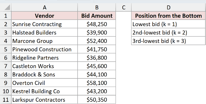
We want to return the lowest, second-lowest, and third-lowest bids without sorting the vendor list.
Here is the formula for the lowest bid:
=SMALL($B$2:$B$11,1)
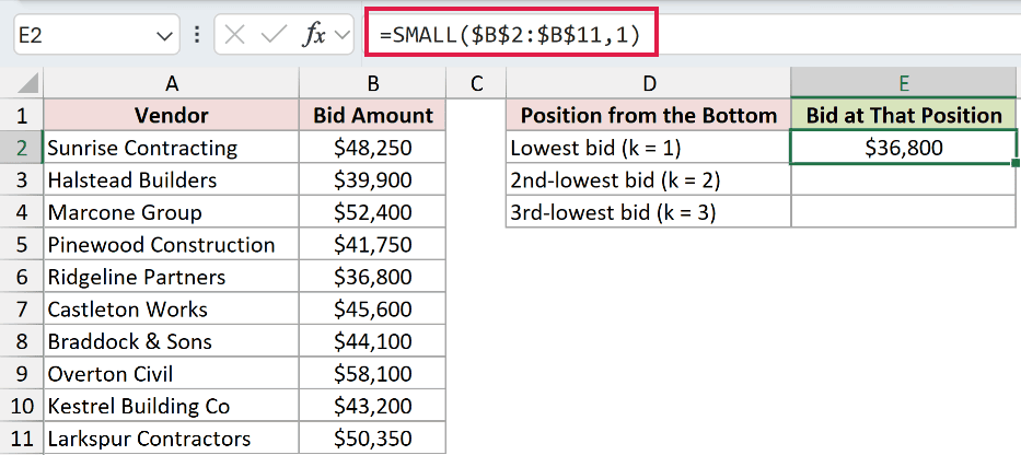
Here is the formula for the second-lowest bid:
=SMALL($B$2:$B$11,2)
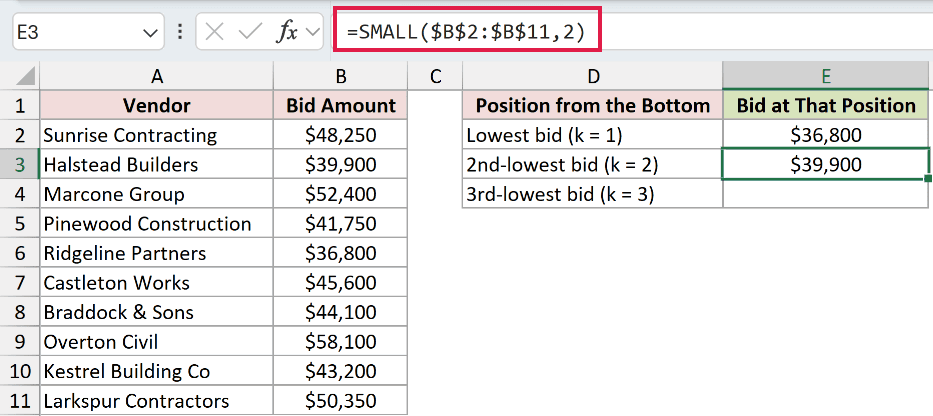
And here is the formula for the third-lowest bid:
=SMALL($B$2:$B$11,3)
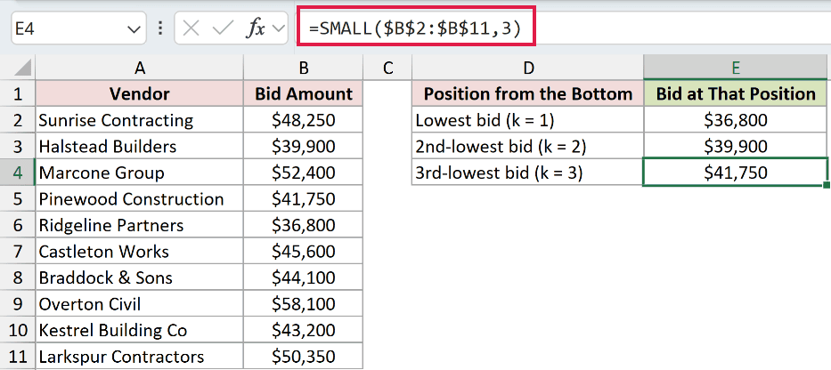
The three formulas change only the k argument. They return $36,800, $39,900, and $41,750 in cells E2, E3, and E4.
MIN can replace the first formula because k is 1. For any later position, SMALL is the more direct choice.
The LARGE function uses the same position logic from the largest end.
Example 2: Return the Bottom Three Bills at Once
One formula can ask SMALL for several positions at once.
Below is the dataset. Columns A and B contain ten branches and their monthly power bills, while columns D and E hold the results.
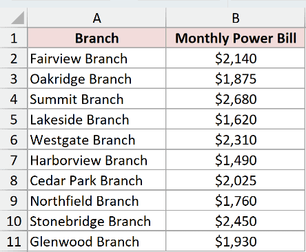
We want the three lowest bills in column D, followed by their total in E2.
Here is the spilling SMALL formula:
=SMALL($B$2:$B$11,SEQUENCE(3))
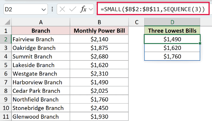
The formula spills $1,490, $1,620, and $1,760 into D2:D4. SEQUENCE supplies the positions 1, 2, and 3 to SMALL.
This spilling approach works in Excel 2021, Excel 2024, and Microsoft 365.
Here is the formula that totals the spilled results:
=SUM(D2#)
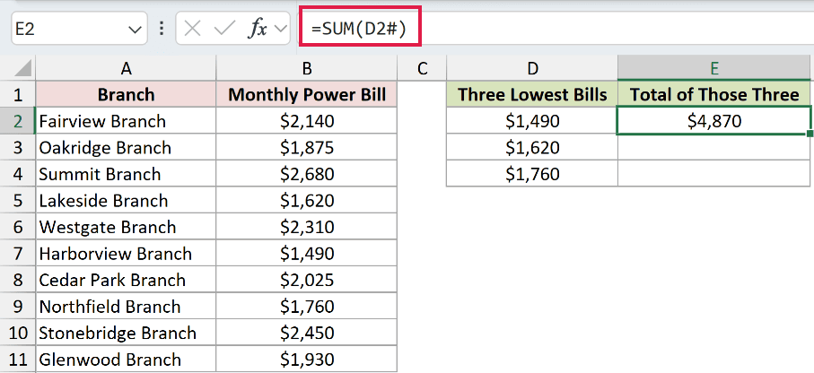
The hash symbol refers to the complete spill beginning in D2. The formula returns $4,870 in E2.
In Microsoft 365 and Excel 2024, =TAKE(SORT($B$2:$B$11),3) is another way to return the bottom three values.
SMALL remains useful when positions come from cells or another formula.
Pro Tip: Keep D2:D4 empty before entering the formula. Any value blocking that output area causes a #SPILL! error.
Example 3: Return the Product Beside a Low Value
Here’s how to return a label instead of the number itself.
Below is the dataset. Columns A and B list eight products and their return rates, while columns D and E compare two lookup methods.
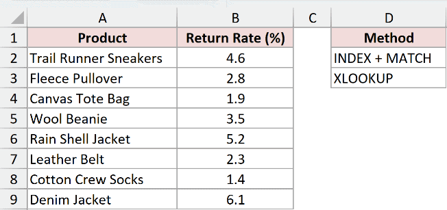
We want the product name associated with the second-lowest return rate.
Here is the INDEX and MATCH formula:
=INDEX($A$2:$A$9,MATCH(SMALL($B$2:$B$9,2),$B$2:$B$9,0))
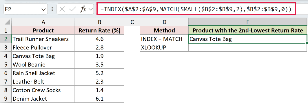
SMALL finds the second-lowest rate. MATCH locates that rate in B2:B9, and INDEX returns the product from the same position in A2:A9.
The result in E2 is Canvas Tote Bag, whose return rate is 1.9.
Here is the XLOOKUP version:
=XLOOKUP(SMALL($B$2:$B$9,2),$B$2:$B$9,$A$2:$A$9)
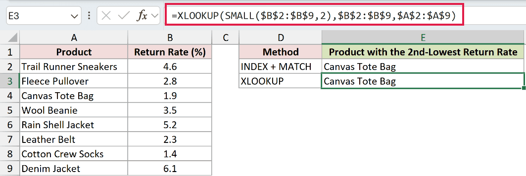
XLOOKUP uses the value returned by SMALL as its lookup value. It also returns Canvas Tote Bag in E3.
XLOOKUP is the shorter option in modern Excel. INDEX and MATCH still work in older versions that don’t include XLOOKUP.
Example 4: Find a Low Value by Condition
A condition can limit the values SMALL evaluates.
Below is the dataset. Columns A:C contain flights, airlines, and fares. Cells E2 and F2 specify Northstar Air and position 2.
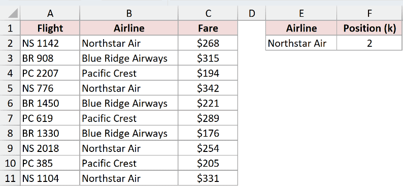
We want the second-lowest Northstar Air fare, using both a modern and a legacy formula.
Here is the formula using FILTER:
=SMALL(FILTER($C$2:$C$11,$B$2:$B$11=$E$2),$F$2)
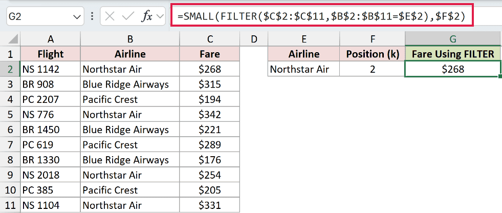
FILTER keeps only fares whose airline matches E2. SMALL then returns the position stored in F2, giving $268 in G2.
Here is the legacy formula using IF:
=SMALL(IF($B$2:$B$11=$E$2,$C$2:$C$11),$F$2)
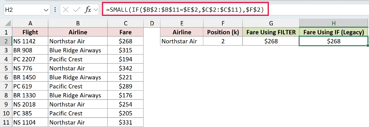
IF passes matching fares to SMALL and leaves FALSE for the other rows. SMALL ignores those logical values and returns $268 in H2.
In Excel 2019 and earlier, enter the IF version with Ctrl + Shift + Enter. In current Excel versions, pressing Enter is enough.
Example 5: Handle Zeros and Tied Values
This dataset shows how zeros and tied values affect each position.
Below is the dataset. Columns A and B show pallets shipped by ten bays. Columns E and F compare results with zeros counted and ignored.
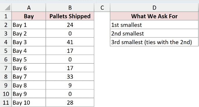
We want the first three positions with zeros included, then the first three nonzero positions.
Here is the formula that counts zeros:
=SMALL($B$2:$B$11,SEQUENCE(3))
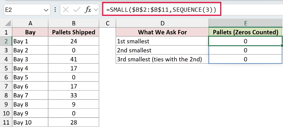
The formula spills 0, 0, and 0 into E2:E4 because three bays contain zero. SMALL treats zero as an ordinary numeric value.
Here is the formula that ignores zeros:
=SMALL(IF($B$2:$B$11<>0,$B$2:$B$11),SEQUENCE(3))
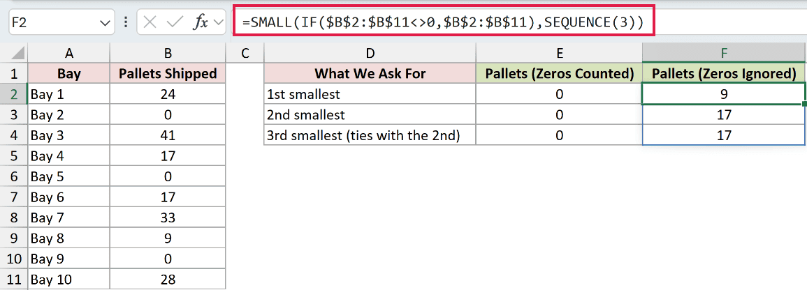
IF passes only nonzero shipments to SMALL. The formula spills 9, 17, and 17 into F2:F4.
The repeated 17 is correct. Bay 4 and Bay 6 each shipped 17 pallets, so that value occupies both the second and third positions.
SMALL works through the sorted list without removing duplicates. If you need the second distinct value, use =SMALL(UNIQUE(range),2).
Example 6: Catch SMALL #NUM! Errors
The last example shows what happens when k falls outside the available positions.
Below is the dataset. Columns A and B contain six batches and defect counts. Column D supplies k, while columns E and F show raw and handled results.
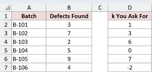
We want SMALL to evaluate each k value, then replace any resulting error with readable text.
Enter this formula in E2 and copy it down through E7:
=SMALL($B$2:$B$7,D2)
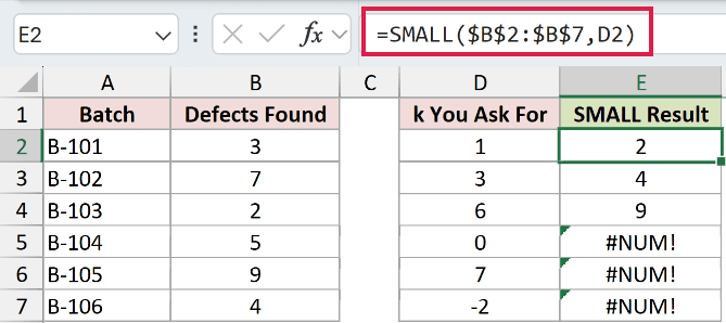
The first three rows return 2, 4, and 9 for k values 1, 3, and 6. Since six numbers exist, k = 6 returns the largest.
The remaining rows use k values 0, 7, and -2. Each returns #NUM! because the requested position is not between 1 and 6.
Enter this formula in F2 and copy it down through F7:
=IFERROR(SMALL($B$2:$B$7,D2),"Not available")
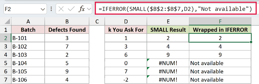
The IFERROR version keeps the valid results as 2, 4, and 9. It displays Not available for the three invalid positions.
Tips & Common Mistakes
- SMALL counts from the bottom, so k must be at least 1 and cannot exceed the number of numeric values. An empty array also produces #NUM!.
=SMALL(range,1)matches MIN, while=SMALL(range,COUNT(range))matches MAX for the same numeric range.- The function ignores text, logical values, and empty cells inside the range. It does not ignore zeros, which can change the position you receive.
- An out-of-range numeric k causes #NUM!. Check the argument itself before troubleshooting the source range.
- SMALL returns one value for one k. Supply several positions with SEQUENCE when you want multiple results to spill.
- Use the spill reference operator in formulas such as
=SUM(D2#)so a calculation follows the complete spilled range. - SMALL can work with FILTER for conditions. If FILTER finds no matching rows, wrap the complete formula in IFERROR when you need a friendlier message.
- LARGE works in the opposite direction. It returns a value by its position from the largest end of the range.
Use SMALL to return a value by its position from the bottom of a range. It can return one ranked value or several positions when paired with a dynamic array.
For conditional lists, filter the values first. For invalid positions, wrap the finished SMALL formula in IFERROR.
Related Excel Functions / Articles:
