REGEXREPLACE Function in Excel

If you want to replace text that follows a pattern, REGEXREPLACE saves you from listing every possible match.

In this article, I’ll show you how to clean and rearrange text, then control which matches Excel replaces.

It is available only in Excel for Microsoft 365 on Windows and Mac.

In Microsoft 365, you can feed REGEXREPLACE a range and the results will spill into the cells below.

REGEXREPLACE Function Syntax in Excel

REGEXREPLACE finds text matching a regular expression, or search pattern, and replaces it with the text you specify.

=REGEXREPLACE(text, pattern, replacement, [occurrence], [case_sensitivity])

• text (required): The text to change, a cell reference, or a range of cells.
• pattern (required): The regular expression that describes what to find. Put a pattern typed directly into the formula inside double quotes.
• replacement (required): The text to insert. Use an empty string, "", to remove matches. You can also reuse captured pieces with $1, $2, and so on.
• occurrence (optional): Which match to replace within each input. The default, 0, replaces all matches. A positive number replaces that numbered match, so 1 replaces the first. A negative number counts from the end, so -1 replaces the last.
• case_sensitivity (optional): Use 0 for case-sensitive matching, which is the default, or 1 to ignore case.

When to Use REGEXREPLACE Function

• Remove unwanted characters when the characters vary between cells.
• Standardize mixed separators and their surrounding spaces.
• Mask part of an identifier while keeping its recognizable ending.
• Rearrange text by capturing pieces and putting them in a different order.
• Replace varying codes or inconsistent capitalization without listing every spelling.

Example 1: Strip Everything Except the Digits

Let’s start with quantities that arrived with extra text attached.

Below is the dataset. Cells A2:A9 contain imported quantities with labels, commas, spaces, and unit descriptions.

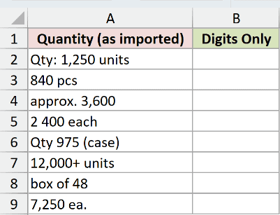
We want to keep only the digits from each quantity.

Here is the formula to enter in B2:

=REGEXREPLACE(A2:A9,"[^0-9]","")

The formula spills through B2:B9, so you don’t need to copy it down.

How this formula works:

• [0-9] describes any digit from 0 to 9.
• The ^ immediately after the opening bracket reverses that selection. So [^0-9] matches any character that isn’t a digit.
• The empty replacement, "", removes each match.
• With occurrence omitted, Excel removes every matching character in each cell.

Qty: 1,250 units becomes 1250, while 2 400 each becomes 2400. The digits stay in their original order.

Pro Tip: These results are text, so Excel may show a green “number stored as text” triangle. Use VALUE around the REGEXREPLACE result when you need numbers for calculations.

This pattern suits whole-number quantities. It also removes decimal points and minus signs, so don’t use it unchanged for decimal or negative amounts.

Example 2: Clean Up Messy Separators in a List

Next, let’s tidy lists where people used different separators.

Below is the dataset. Cells A2:A9 contain skill lists with commas, semicolons, repeated separators, and inconsistent spacing.

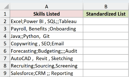
We want one comma followed by one space between each listed skill.

Here is the formula to enter in B2:

=REGEXREPLACE(A2:A9,"\s*[;,]+\s*",", ")

The results spill into B2:B9. For example, Java;;Python, Git becomes Java, Python, Git.

How this formula works:

• \s* matches zero or more whitespace characters before a separator.
• [;,]+ matches one or more consecutive semicolons or commas.
• The final \s* includes any whitespace immediately after those separators.
• The replacement ", " puts back one comma and one space.

The same pattern turns Forecasting;Budgeting;;;Audit into Forecasting, Budgeting, Audit without changing the skill names.

TRIM alone can’t standardize commas and semicolons. SUBSTITUTE would need multiple replacements, while this pattern handles the separator variations shown here in one pass.

Example 3: Mask All But the Last 4 Digits

Now let’s keep the recognizable ending of each employee identifier.

Below is the dataset. Column A lists employees, and B2:B9 contains Tax IDs in a consistent three-digit, two-digit, four-digit format.

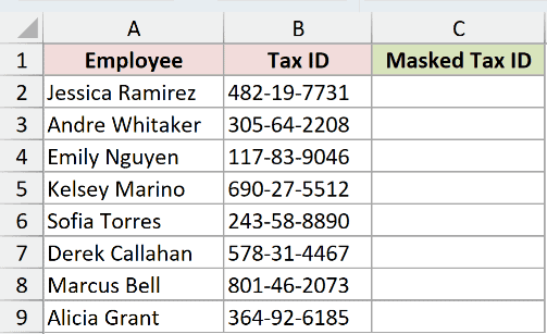
We want to replace the first five digits with asterisks and leave the last four visible.

Here is the formula to enter in C2:

=REGEXREPLACE(B2:B9,"\d{3}-\d{2}","***-**")

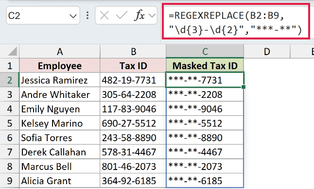
The masked identifiers spill into C2:C9. Jessica Ramirez’s result is ***-**-7731, and Andre Whitaker’s is ***-**-2208.

How this formula works:

• \d{3} matches three digits.
• The hyphen matches the hyphen between the first two groups.
• \d{2} matches the next two digits.
• "***-**" replaces that matched section, leaving the final hyphen and four digits untouched.

The asterisks are replacement text here. They aren’t acting as search instructions.

REPLACE is also suitable when positions are fixed like these. This REGEXREPLACE pattern specifically expects the three-digit group, hyphen, and two-digit group.

Pro Tip: The original IDs remain in column B. For a report that should contain only masked IDs, copy the masked results as values into a separate file without the source IDs.

Example 4: Rearrange a Date With Capture Groups

Here’s where matching a pattern also lets you reuse what it finds.

Below is the dataset. Cells A2:A9 contain imported text dates in MM/DD/YYYY format, with two-digit months and days.

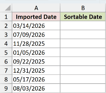
We want to rearrange each text date into YYYY-MM-DD order.

Here is the formula to enter in B2:

=REGEXREPLACE(A2:A9,"(\d{2})/(\d{2})/(\d{4})","$3-$1-$2")

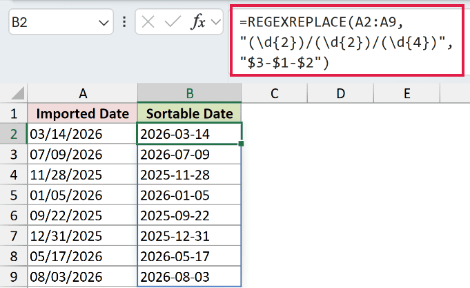
The results spill through B2:B9. The first date, 03/14/2026, becomes 2026-03-14.

How this formula works:

• Parentheses create capture groups, which remember the matched text for reuse.
• The first (\d{2}) captures the month. The second captures the day.
• (\d{4}) captures the year as the third group.
• "$3-$1-$2" inserts the year, month, and day in that order, separated by hyphens.

For 11/28/2025, the result is 2025-11-28. These consistently formatted text strings can sort in chronological order because the year comes first.

Pro Tip: The output is still text, not a real Excel date. Changing its number format won’t convert it. Convert it to a date value before using date arithmetic.

This pattern expects two digits for both month and day. It rearranges the matching text; it doesn’t check whether that text represents a valid calendar date.

Example 5: Replace Every Match or the First

Let’s compare replacing every code with replacing only the first one.

Below is the dataset. Cells A2:A8 contain promotional messages with repeated codes and codes whose digits differ within the same message.

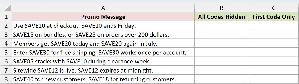
We want to compare hiding all matching codes with hiding only the first code in each message.

Here is the formula to enter in B2 for all matches:

=REGEXREPLACE(A2:A8,"SAVE\d+","[CODE]")

And here is the formula to enter in C2 for the first match only:

=REGEXREPLACE(A2:A8,"SAVE\d+","[CODE]",1)

The formulas spill into B2:B8 and C2:C8. Both use SAVE\d+ to match SAVE followed by one or more digits.

The first formula omits occurrence, so it replaces every match. The second sets occurrence to 1, which restarts the count for each input cell.

In B2, the result is Use [CODE] at checkout. [CODE] ends Friday.

In C2, it is Use [CODE] at checkout. SAVE10 ends Friday.

The distinction also holds when the codes differ. Cell C6 returns [CODE] stacks with SAVE10 during clearance week.

SUBSTITUTE also has an instance_num argument for replacing only the first occurrence. REGEXREPLACE earns its place here because SAVE05, SAVE10, and the other codes vary.

A single literal SUBSTITUTE replacement wouldn’t match all those codes. The pattern does.

Example 6: Ignore Case When Replacing Text

Finally, let’s fix inconsistent capitalization in payment notes.

Below is the dataset. Cells A2:A8 contain payment notes with different capitalizations of the same payment service name.

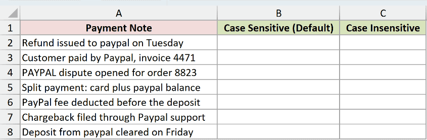
We want to standardize the name’s capitalization while keeping the rest of each note unchanged.

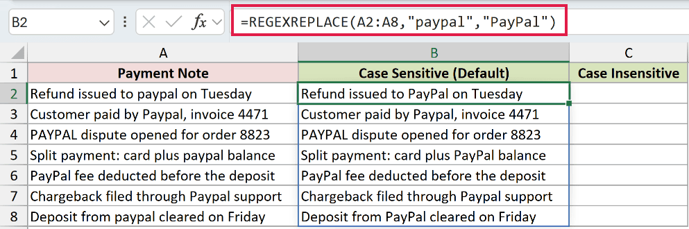
Here is the formula to enter in B2 using the case-sensitive default:

=REGEXREPLACE(A2:A8,"paypal","PayPal")

And here is the formula to enter in C2 to ignore case:

=REGEXREPLACE(A2:A8,"paypal","PayPal",0,1)

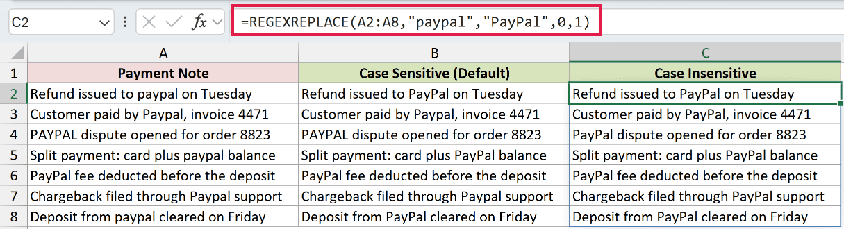
The results spill into B2:B8 and C2:C8. The default matches only the exact lowercase spelling supplied in the pattern.

Cell B3 therefore remains Customer paid by Paypal, invoice 4471. Cell C3 returns Customer paid by PayPal, invoice 4471.

The difference is clear in row 4 too. Cell B4 retains PAYPAL dispute opened for order 8823.

Cell C4 instead returns PayPal dispute opened for order 8823.

In the second formula, 0 means replace every occurrence, and the final 1 turns on case-insensitive matching. Don’t swap those argument positions.

SUBSTITUTE is case sensitive and has no equivalent flag. You’d need separate replacements for the different spellings to get the same cleanup.

Tips & Common Mistakes

• Check your Excel version. REGEXREPLACE requires Excel for Microsoft 365 on Windows or Mac. It isn’t available in Excel 2021 or Excel 2024.
• Keep the spill area empty. These range-based formulas return one text result per input cell. If another value blocks the output area, Excel returns #SPILL!.
• Edit the starting cell. Change a spilled formula in its top cell. Adding @ introduces implicit intersection and can reduce a range-based result to one value.
• Remember the defaults. Omitting the final two arguments replaces every match and treats uppercase and lowercase letters as different.
• Expect unchanged text when nothing matches. Example 6’s default formula leaves differently capitalized spellings untouched. Check the pattern before assuming the formula failed.
• Keep text results in mind. Digit-only output isn’t automatically numeric, and rearranging a date string doesn’t create a date value.
• Choose the tool for the job. Use SUBSTITUTE for a literal text replacement, REPLACE for fixed character positions, REGEXEXTRACT to pull matching text out, and REGEXTEST to check for a match.

Start with the example whose pattern fits your data, then check a few varied rows before using it across the full list.

Keep the original text beside the result while checking. It’s easier to spot an overly broad match when you can compare both.

List of All Excel Functions