REPLACE Function in Excel (6 Easy Examples)

If you want to swap out characters at a specific spot in a text string, like the first two letters of a code or the digits in the middle of a card number, the REPLACE function is what you’re looking for.

The key thing to know is that REPLACE works by position. You tell it where to start and how many characters to swap, not which text to find. In this article, I’ll show you how to use it with six practical examples.

In Excel 365, you can also feed REPLACE a range and the results will spill into the cells below.

Table of Contents

REPLACE Function Syntax in Excel

The REPLACE function replaces part of a text string with a different string, based on the position and number of characters you specify.

=REPLACE(old_text, start_num, num_chars, new_text)

old_text – the original text string you want to change.
start_num – the position of the first character you want to replace.
num_chars – how many characters to replace, starting from start_num.
new_text – the text that goes in place of the removed characters.

When to Use REPLACE Function

Here are some common situations where REPLACE comes in handy:

Swapping a fixed prefix or code at the start of every entry.
Inserting text at a known position without deleting anything (set num_chars to 0).
Masking part of a sensitive number, like a credit card or account number.
Cleaning up or removing a fixed-length chunk from the start of a string.
Reformatting raw strings, such as turning a plain date string into a dashed format.

Example 1: Replace Characters at a Fixed Position

Let’s start with a simple case where the position is always the same.

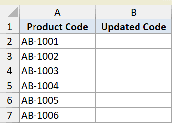
Below is the dataset. Column A has a list of product codes that all begin with the prefix “AB”.

Excel dataset with Product Code in column A and empty Updated Code column B for REPLACE function example

Say you want to change that “AB” prefix to “XY” for every code, keeping the rest of each code as it is.

Here is the formula:

=REPLACE(A2:A7,1,2,"XY")

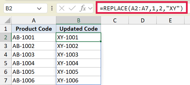
This starts at position 1 and replaces 2 characters with “XY”. So “AB-1001” becomes “XY-1001”, and the rest of the string stays untouched.

Since this is entered in Excel 365, one formula handles the whole column. The results spill down automatically from B2.

Example 2: Insert Text Without Removing Any (num_chars 0)

Here’s a handy trick. If you set num_chars to 0, REPLACE inserts text without deleting anything.

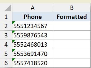
Below is the dataset. Column A has phone numbers stored as plain 10-digit strings.

Excel dataset for REPLACE function showing a list of unformatted phone numbers in column A and empty column B

Say you want to add a “+1 ” country code prefix in front of each number without losing a single digit.

Here is the formula:

=REPLACE(A2:A6,1,0,"+1 ")

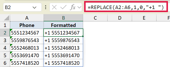
Excel formula bar showing REPLACE function adding +1 prefix to phone numbers in a formatted column

Because num_chars is 0, nothing gets removed. The “+1 ” is simply inserted at position 1, pushing the original number to the right.

Pro Tip: Setting num_chars to 0 turns REPLACE into an insert tool. It’s perfect for adding a prefix, a separator, or any text at a fixed spot without disturbing the original string.

Example 3: Remove Characters by Replacing With Nothing

You can also use REPLACE to delete characters. The trick is to replace them with an empty string.

Below is the dataset. Column A has invoice IDs that all start with the prefix “INV-“.

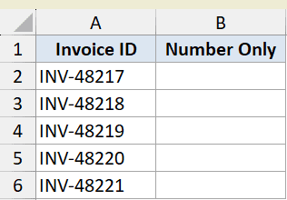
Excel dataset for REPLACE function example showing Invoice IDs in column A and empty Number Only cells in column B

Say you want to strip off that 4-character “INV-” prefix and keep only the number part.

Here is the formula:

=REPLACE(A2:A6,1,4,"")

Excel formula bar showing REPLACE function to extract numbers from invoice IDs in column B

This starts at position 1, replaces 4 characters, and puts an empty string (“”) in their place. So “INV-48217” becomes “48217”.

This is one of the cleanest ways to chop off a fixed-length chunk from the start of a string. It’s also the basis for a quick way to remove the first character in Excel.

Example 4: Mask Part of a Number for Privacy

A really common use of REPLACE is hiding sensitive digits, like the middle of a credit card number.

Below is the dataset. Column A has full card numbers in the format 4532-1234-5678-9012.

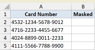
Excel dataset for REPLACE function showing Card Number in column A and empty Masked column B

Say you want to keep the first block visible but mask the middle, showing something like 4532-XXXX-XXXX-9012.

Here is the formula:

=REPLACE(A2:A5,6,9,"XXXX-XXXX")

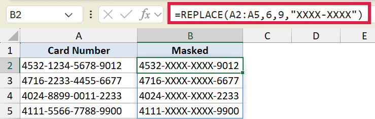
This starts at position 6 (right after the first dash) and replaces the next 9 characters with “XXXX-XXXX”. The first and last blocks stay visible while the middle is hidden.

Pro Tip: REPLACE only works when the characters you want to mask are always in the same position. If your numbers vary in length or format, count the positions carefully or use a FIND-based approach like in the next example.

Example 5: Replace at a Position Found by FIND

So far the position has been fixed. But what if it changes from row to row? You can let the FIND function locate the spot for you.

Below is the dataset. Column A has email addresses that all use the “@oldcorp.com” domain.

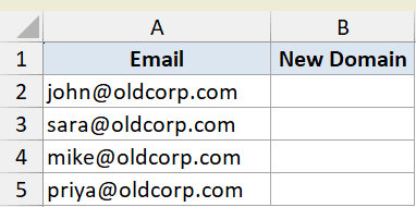
Excel dataset showing email addresses in column A and an empty New Domain column B for REPLACE function example 5

Say you want to swap every domain to “newco.com” while keeping each person’s username intact. The username length varies, so the start position is different on each row.

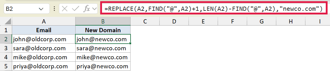
Here is the formula:

=REPLACE(A2,FIND("@",A2)+1,LEN(A2)-FIND("@",A2),"newco.com")

Excel formula bar highlighting REPLACE function to change email domain to newco.com in column B

Here is how this formula works:

FIND(“@”,A2)+1 finds the “@” and adds 1, so the start position is the first character after the “@”.
LEN(A2)-FIND(“@”,A2) counts how many characters come after the “@”, which is the length we need to replace.
“newco.com” is the new domain that goes in.

Because the start position and length are calculated per row, you fill this formula down B2:B5 rather than spilling it. That keeps each row’s FIND and LEN reading clearly.

In Excel 365, you can also do this more directly with TEXTBEFORE: =TEXTBEFORE(A2,"@")&"@newco.com". That grabs the username before the “@” and tacks on the new domain. The REPLACE + FIND version still works (and works in older Excel where TEXTBEFORE doesn’t exist), so it’s worth knowing both.

Example 6: Nested REPLACE to Format a Raw String

You can nest one REPLACE inside another when you need to make more than one change at known positions.

Below is the dataset. Column A has dates stored as plain 8-digit strings in YYYYMMDD format.

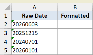
Excel dataset for replace example 6 showing raw date strings in column A and empty formatted cells in column B

Say you want to turn “20260603” into “2026-06-03” by inserting a dash after the year and another after the month.

Here is the formula:

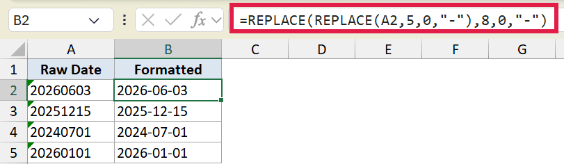
=REPLACE(REPLACE(A2,5,0,"-"),8,0,"-")

Excel formula bar showing nested REPLACE functions to format raw date strings into YYYY-MM-DD format in cell B2

Here is how this formula works:

The inner REPLACE inserts a dash at position 5, turning “20260603” into “2026-0603”.
The outer REPLACE then inserts a dash at position 8 of that new string, giving “2026-06-03”.

Notice the outer position is 8, not 7. That’s because the first dash already pushed every character after it one spot to the right. Always count positions on the string as it exists at each step.

Tips & Common Mistakes

REPLACE works by position, SUBSTITUTE works by matching text. Use REPLACE when you know exactly where the characters sit. If you instead want to find and swap specific text wherever it appears, the SUBSTITUTE function is the better fit.
num_chars set to 0 inserts instead of replaces. This is the easiest way to add a prefix or separator without losing any of the original text.
Replace with “” to delete. An empty string as new_text removes the characters in that range, which is handy for trimming fixed-length prefixes.
Watch your positions in nested REPLACE. Each insert shifts the characters after it, so the second position has to account for what the first one added.
A #SPILL! error means the output is blocked. When you use the spilling form in Excel 365, make sure the cells below the formula are empty so the results have room to fill in.

REPLACE is one of those text functions that feels limited at first but quietly solves a lot of cleanup jobs. Once you get comfortable counting positions, you can swap prefixes, mask sensitive data, insert separators, and reformat raw strings in a single formula.

It pairs well with other text tools too, so it’s worth knowing how to extract part of text in a cell when REPLACE isn’t quite the right fit.

The main thing to remember is the by-position vs by-matching distinction. Reach for REPLACE when position is what you know, and reach for SUBSTITUTE when the text itself is what you’re matching.

List of All Excel Functions

Related Excel Functions / Articles: