If you want to locate the position of a character or piece of text inside a cell, the FIND function is what you need.
In this article, I’ll show you five practical examples of how to use FIND on its own and combined with other functions like LEFT and MID.
In Excel 365 you can give FIND a whole range and the positions spill down the column, for example =FIND("@",A2:A7).
FIND Function Syntax in Excel
Here is the syntax for the FIND function:
=FIND(find_text, within_text, [start_num])
- find_text – the character or text you want to locate. FIND is case-sensitive, and wildcards are not supported.
- within_text – the text to search inside. Usually a cell reference.
- [start_num] – where to start the search (default is 1). Set this past the first match to find a later occurrence.
If FIND cannot find the text, it returns a #VALUE! error. Use SEARCH instead when case does not matter.
When to Use FIND Function
- Get the position of a delimiter (like
-or@) to feed into LEFT, MID, or RIGHT for text extraction. - Do case-sensitive matching, since SEARCH ignores case but FIND does not.
- Find the second or Nth occurrence of a character by using the
start_numargument to skip past the first one. - Test whether a cell contains certain text with
=ISNUMBER(FIND(...)). See the ISNUMBER function for more on that pattern.
Example 1: Find the Position of a Character
Let’s start with a simple example.
Below is a list of product codes in column A. Each code uses a dash as a separator, and we want to know the position of the first dash in each code.
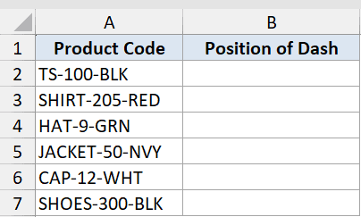
We want to find the position of the first dash in each product code.
Here is the formula:
=FIND("-",A2)
The formula scans the text in A2 and returns the position of the first -, counting from 1. Since the product codes have different-length prefixes, the results vary. TS-100-BLK gives 3, SHIRT-205-RED gives 6, and HAT-9-GRN gives 4.
FIND always returns the position of the first match. For more ways to find the position of a character in a string, including Nth-occurrence patterns, check that linked guide.
Pro Tip: To find the second dash, use the optional third argument. For example, =FIND(“-“,A2,FIND(“-“,A2)+1) starts the search right after the first dash.
Example 2: FIND vs SEARCH (Case Sensitivity)
Here’s a practical scenario to show what makes FIND unique.
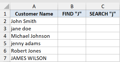
Below we have a list of customer names in column A. We want to search for the capital letter “J” using both FIND and SEARCH so you can see exactly how they differ.
We want to compare how FIND and SEARCH handle the same search term when the case doesn’t match.
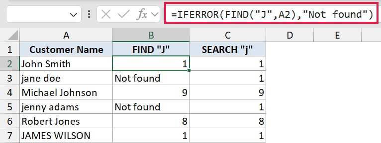
Here is the formula for the FIND column (column B):
=IFERROR(FIND("J",A2),"Not found")
And for the SEARCH column (column C):
=IFERROR(SEARCH("j",A2),"Not found")
How this formula works:
- FIND looks for a capital “J”. “John Smith” returns 1, but “jane doe” returns “Not found” because there is no uppercase J.
- SEARCH ignores case, so it finds the j in every name regardless of how it is typed.
- IFERROR wraps both formulas to replace the
#VALUE!error with a clean “Not found” message.
Use FIND when case matters. Use SEARCH when it does not. For a full side-by-side comparison, see SEARCH vs FIND in Excel.
Example 3: Extract Text Before a Character
Let’s try something more useful: pulling out just part of a cell’s text.
Below is a list of email addresses. We want to extract just the username, which is everything before the @ symbol.
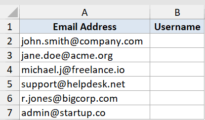
We want to pull the username portion out of each email address.
Here is the formula:
=LEFT(A2,FIND("@",A2)-1)
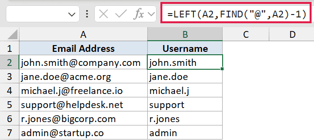
How this formula works:
FIND("@",A2)returns the position of the@sign. For john.smith@company.com that is 11.- Subtracting 1 gives us 10, which is the number of characters before the
@. LEFT(A2,10)then pulls exactly those 10 characters, giving usjohn.smith.
In Excel 365, the TEXTBEFORE function does the same job in one step: =TEXTBEFORE(A2,"@"). That is more direct, but the LEFT + FIND version still works in older Excel versions where TEXTBEFORE is not available.
Example 4: Extract Text After a Character
Here’s the flip side of the previous example.
Below is a list of full names in column A. We want to extract just the last name, which comes after the space.
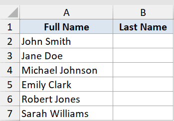
We want to pull the last name from each full name.
Here is the formula:
=MID(A2,FIND(" ",A2)+1,100)
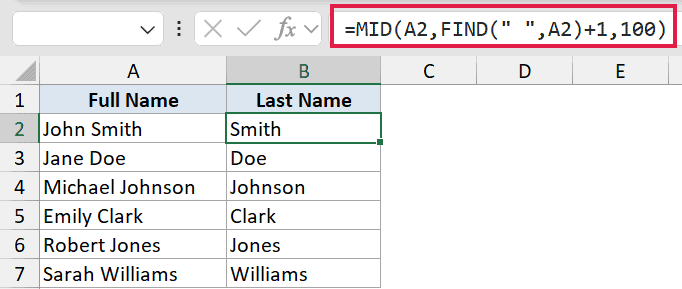
How this formula works:
FIND(" ",A2)locates the position of the space. For “John Smith” that is 5.- Adding 1 moves us to position 6, which is where the last name starts.
MID(A2,6,100)extracts from position 6 for up to 100 characters. The 100 is just a generous number to grab everything to the end.
In Excel 365, =TEXTAFTER(A2," ") does the same thing in one step. The MID + FIND version still works everywhere, including older Excel, so it is worth knowing both. For more text extraction techniques, see how to extract part of text in Excel.
Example 5: Spill Positions for a Whole Column
Now let’s take advantage of Excel 365’s dynamic arrays.
Below is a mix of email addresses and one row without an email. We want to find the @ position for every row at once, with a single formula.
We want one formula to return the @ position for all six rows, and return a blank for any row that has no @.
Here is the formula:
=IFERROR(FIND("@",A2:A7),"")
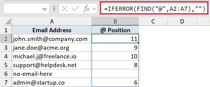
Enter this in cell B2 and it spills results down to B7 automatically. FIND processes each cell in the range A2:A7 and returns a separate position value for each one.
The row with “no-email-here” has no @, so FIND would return #VALUE! for that row. IFERROR catches it and returns an empty string instead.
Pro Tip: In older versions of Excel (pre-365), this spilling behavior is not available. You would need to enter =IFERROR(FIND(“@”,A2),””) in B2 and drag the formula down the column manually.
Tips & Common Mistakes
- FIND is case-sensitive. If you search for “j” and the cell has “J”, FIND returns
#VALUE!. Switch to SEARCH if you want a case-insensitive match. - #VALUE! when text is not found. FIND does not return a zero or blank – it throws an error. Always wrap FIND in IFERROR if the search text might not be present.
- No wildcards. FIND does not support
*or?as wildcards. Use SEARCH for wildcard matching. - Finding a later occurrence. Use the optional
start_numargument to skip past an earlier match. For the second dash in “TS-100-BLK”, use=FIND("-",A2,FIND("-",A2)+1). - Testing for text. To check whether a cell contains a certain string, use
=ISNUMBER(FIND("text",A2)). This returns TRUE when the text is found and FALSE when it is not, with no error.
FIND is a simple but powerful function once you know how to pair it with LEFT, MID, and IFERROR. Whether you need to extract text from delimited strings or do case-sensitive checks, FIND gives you the precise position control you need.
Related Excel Functions / Articles: