LEFT Function in Excel (6 Easy Examples)

If you want to pull the first few characters from the start of a text string, like a product prefix, a first name, or the part of an email before the @, the LEFT function is what you’re looking for.

It grabs characters counting from the left side of any cell. In Excel 365, you can also feed LEFT a whole range and the results spill into the cells below.

In this article I will show you how to use the LEFT function in Excel using 6 practical examples.

Table of Contents

LEFT Function Syntax in Excel

Here is how the LEFT function is written.

=LEFT(text, [num_chars])

text – the text string you want to extract characters from. This can be a cell reference or text typed directly in quotes.
num_chars – optional. How many characters to pull from the left. If you leave it out, LEFT returns just the first character.

When to Use LEFT Function

Pulling a fixed-length prefix off a code, like the first 3 letters of a product ID.
Grabbing a first name out of a full name field.
Extracting the username portion of an email address.
Stripping a unit label (like “kg”) off the end so you keep the number part.
Splitting an ID and a status that are joined by a dash or other separator.

Example 1: Extract the First Few Characters

Let’s start with the simplest use of LEFT, pulling a fixed number of characters off the front.

Below is the dataset. Column A has product codes, and column B is where we want the category prefix to land.

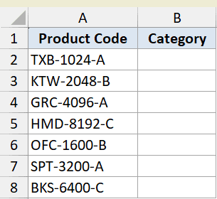
Excel dataset showing Product Code in column A with alphanumeric codes and an empty Category column B

We want the first 3 characters of each code, which is the category prefix.

Here is the formula:

=LEFT(A2:A8,3)

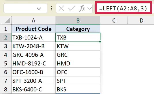
Excel formula bar showing =LEFT(A2:A8,3) to extract the first three characters of product codes into column B

The second argument, 3, tells LEFT to grab three characters starting from the left. So “TXB-1024-A” becomes “TXB”.

Notice we fed the whole range A2:A8 into one formula in cell B2. In Excel 365, the result spills down automatically, so you don’t need to copy the formula to each row.

Pro Tip: If you only need the first character, you can skip the second argument entirely. LEFT defaults to 1 when num_chars is left out.

Example 2: Get the First Character Only

Here’s a case where the default behavior of LEFT does the work for us.

Below is the dataset. Column A has size labels where the first character is the size code, like “S – Small”.

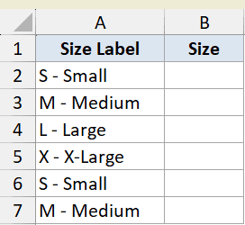
Excel dataset for LEFT function example 2 with Size Label in column A and empty Size column B

We want just the single-letter size code from each label.

Here is the formula:

=LEFT(A2:A7)

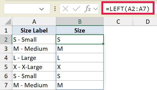
Excel formula =LEFT(A2:A7) extracting the first character from Size Label column A into Size column B

There’s no second argument here. When you skip num_chars, LEFT assumes you want one character. So “S – Small” returns “S”.

This is handy any time the value you need sits in the very first position of the string.

Example 3: Extract the First Name

Now let’s pull a name out of a field, where the number of characters changes from row to row. This is one common way to extract a first name in Excel.

Below is the dataset. Column A has full names with a first name, a space, and a last name.

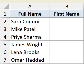
Excel dataset for LEFT function with Full Name in column A and empty First Name cells in column B

We want everything before the first space, which is the first name.

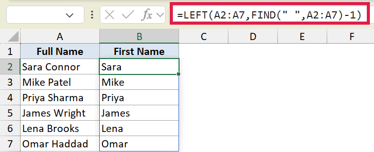
Here is the formula:

=LEFT(A2:A7,FIND(" ",A2:A7)-1)

Excel formula using LEFT and FIND functions to extract first names from a list of full names in column A to column B

Here is how this formula works.

FIND(” “, A2:A7) returns the position of the first space in each name.
We subtract 1 so we stop just before the space.
LEFT then pulls that many characters from the left.

So for “Sara Connor”, the space is at position 5, we subtract 1 to get 4, and LEFT returns “Sara”.

In Excel 365, you can also do this with TEXTBEFORE: =TEXTBEFORE(A2:A7," "). That’s more direct than the LEFT plus FIND approach. The LEFT version still works, and works in older Excel versions where TEXTBEFORE doesn’t exist, so it’s worth knowing both.

Example 4: Get the Username From an Email

Email addresses are an easy one for LEFT, since the part you want ends at a known character.

Below is the dataset. Column A has email addresses, and we want the username that comes before the @ sign.

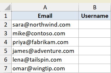
Excel dataset for LEFT function tutorial showing a list of email addresses in column A and empty Username cells in column B

We want everything to the left of the @ in each address.

Here is the formula:

=LEFT(A2:A7,SEARCH("@",A2:A7)-1)

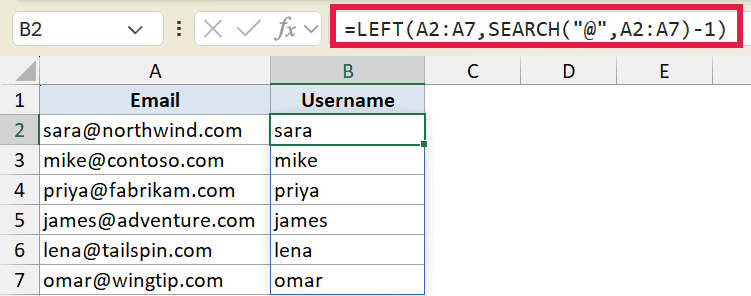
Excel formula using LEFT and SEARCH to extract usernames from email addresses in column A to column B

SEARCH finds the position of the @ symbol, we subtract 1, and LEFT grabs that many characters. So “sara@northwind.com” returns “sara”.

You could use FIND here instead of SEARCH and get the same result. The difference is that SEARCH ignores case, while FIND is case-sensitive.

Pro Tip: In Excel 365 you can get the same result with `=TEXTBEFORE(A2:A7,”@”)`, which skips the position math entirely. The SEARCH version still works in older Excel versions.

Example 5: Remove the Last Few Characters

Sometimes you don’t know the prefix length, but you do know how many characters to chop off the end. LEFT pairs with LEN here, the same trick used to remove the last 4 characters in Excel.

Below is the dataset. Column A has weight measurements with a ” kg” unit at the end, like “1500 kg”.

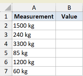
Excel LEFT function example 5 dataset showing column A with measurement values in kg and empty column B

We want to drop the last 3 characters, which is the space and “kg”, and keep the number.

Here is the formula:

=LEFT(A2:A7,LEN(A2:A7)-3)

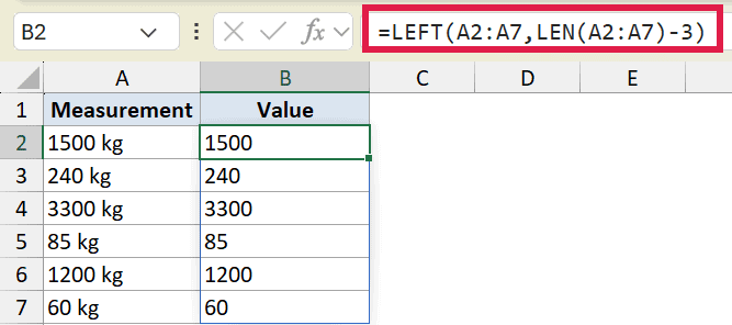
Excel formula =LEFT(A2:A7, LEN(A2:A7)-3) used to extract numeric values from column A into column B

LEN counts the total characters in the string. We subtract 3 to account for the space and the two letters in “kg”. LEFT then keeps everything except those last 3 characters.

So “1500 kg” has 7 characters, minus 3 leaves 4, and LEFT returns “1500”.

Example 6: Split Out a Number Before a Dash

This last example pulls a number out of a tag and converts it into a real number you can do math with.

Below is the dataset. Column A has invoice tags joining an amount and a status with a dash, like “450-PAID”.

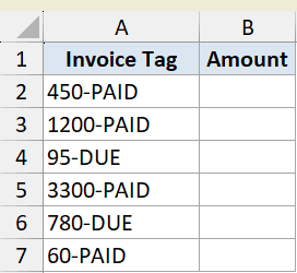
Excel dataset for LEFT function example showing Invoice Tags like 450-PAID and 1200-PAID in column A

We want the amount before the dash, returned as an actual number rather than text.

Here is the formula:

=VALUE(LEFT(A2:A7,FIND("-",A2:A7)-1))

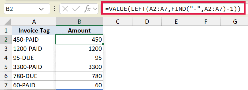
Excel formula using LEFT and FIND to extract numeric amounts from invoice tags in column A to column B

Here is how this formula works.

FIND locates the dash, and we subtract 1 to stop just before it.
LEFT pulls the digits ahead of the dash, but they come back as text.
VALUE wraps the result and turns that text into a real number.

So “450-PAID” gives the text “450”, and VALUE converts it to the number 450 that you can sum or sort.

In Excel 365, you could pull the text part with =TEXTBEFORE(A2:A7,"-") and still wrap it in VALUE. The FIND version works in older versions too, so keep both in your back pocket.

Tips & Common Mistakes

LEFT always returns text, even when the characters are digits. If you need to add, sort, or compare the result as a number, wrap it in VALUE like in Example 6.
SEARCH is case-insensitive and supports wildcards, while FIND is case-sensitive. Pick FIND when case matters, SEARCH when it doesn’t.
If you only want the first character, skip the num_chars argument. LEFT defaults to 1.
Feeding a range into one LEFT formula in Excel 365 spills the results automatically, so there’s no need to copy the formula down each row.
To split a string into multiple columns at once instead of just the left piece, look at TEXTSPLIT in Excel 365.

LEFT is one of those small functions you’ll reach for all the time once you know it. On its own it pulls a fixed number of characters off the front. Pair it with FIND, SEARCH, or LEN and it handles names, usernames, and codes of any length.

List of All Excel Functions

Related Excel Functions / Articles: