
The MINIFS function in Excel returns the smallest number from cells that meet all the conditions you specify.
You can find the lowest price for a supplier or the earliest date for a category without first filtering the source data.
In this article, I’ll show you how to find minimums with multiple criteria, exclude zeros, and calculate minimums for each group.
MINIFS Function Syntax in Excel
The MINIFS function finds the smallest number in a range after applying one or more conditions.
=MINIFS(min_range, criteria_range1, criteria1, [criteria_range2, criteria2], ...)
- min_range (required) contains the numbers from which Excel returns the minimum.
- criteria_range1 (required) contains the values tested by the first condition.
- criteria1 (required) defines the first condition.
- criteria_range2, criteria2 (optional) add further conditions. You can supply up to 126 criteria pairs, and every pair must match on the same row.
When to Use MINIFS Function
- Find the lowest price, rate, score, or quantity for one category.
- Apply several conditions when every condition must be true on the same row.
- Use comparison operators or wildcards inside criteria.
- Exclude zero values from a minimum calculation.
- Find a minimum for each item in a spilled list.
Example 1: MINIFS With One Criterion
Let’s start with a supplier quote table and one straightforward condition.
Below is the dataset. Columns A through D contain quote details, while F2 holds the Hydraulic Pump criterion.
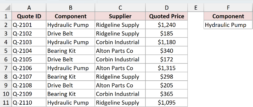
We want the lowest quoted price for the component entered in F2.
Here is the formula:
=MINIFS(D2:D11,B2:B11,F2)
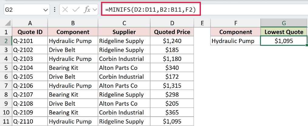
Excel checks B2:B11 for Hydraulic Pump, then finds the smallest matching value in D2:D11. The result in G2 is $1,095.
MINIFS returns the price, not the supplier’s name. You can use XLOOKUP or INDEX and MATCH when you also need the related record.
Example 2: MINIFS With Multiple Criteria
Now let’s add a second condition to a freight rate comparison.
Below is the dataset. Columns A through D list the freight quotes, while F2 and G2 contain the lane and service criteria.
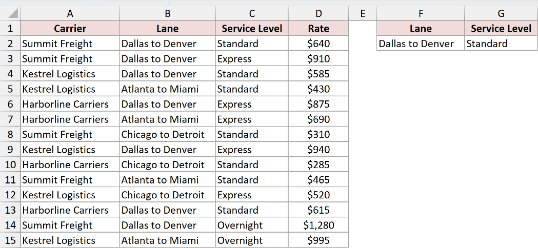
We want the lowest Standard rate for the Dallas to Denver lane.
Here is the formula:
=MINIFS(D2:D15,B2:B15,F2,C2:C15,G2)
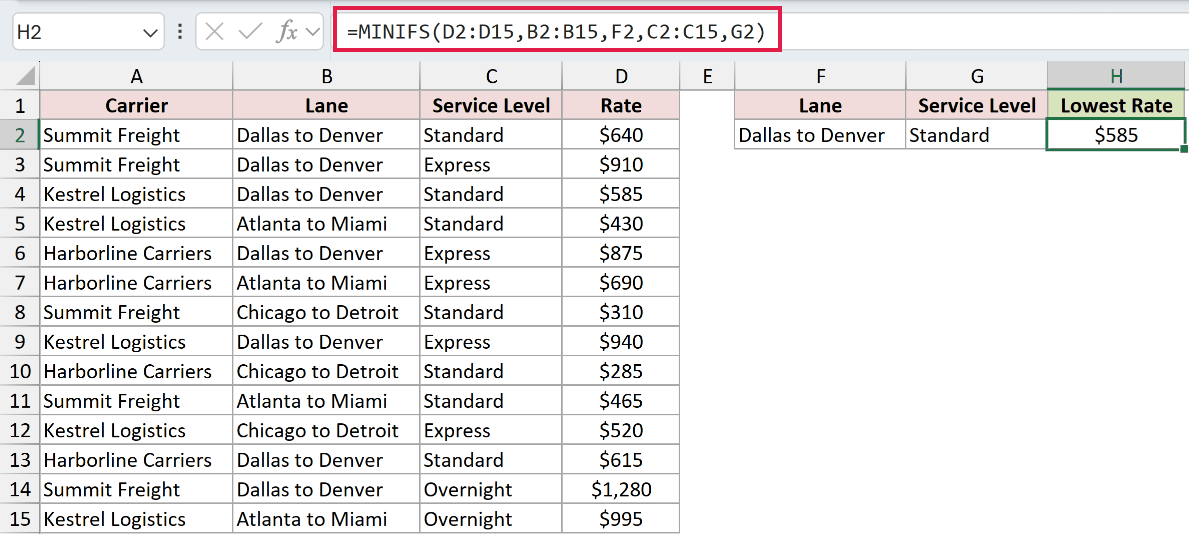
The first pair tests the lane in column B. The second tests the service level in column C.
Both conditions must be true on the same row. The lowest qualifying rate in H2 is $585.
Pro Tip: MINIFS combines criteria with AND logic. For OR logic, use MIN with FILTER in Excel 2021 and later.
Example 3: MINIFS With Operators and Wildcards
Here’s how to build more flexible criteria for a rental listing table.
Below is the dataset. Columns A through D hold each listing, unit type, bedroom count, and rent. F2 contains the minimum bedroom count.
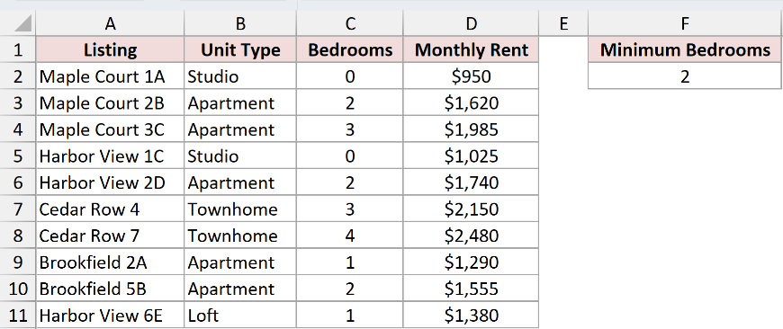
First, we want the cheapest listing with at least the number of bedrooms entered in F2.
Here is the formula:
=MINIFS(D2:D11,C2:C11,">="&F2)
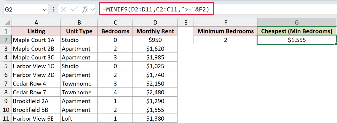
The operator is text, so ">="&F2 joins it to the value in F2. With F2 set to 2, G2 returns $1,555.
Next, we want the cheapest listing that isn’t a Studio.
Here is the formula:
=MINIFS(D2:D11,B2:B11,"<>Studio")
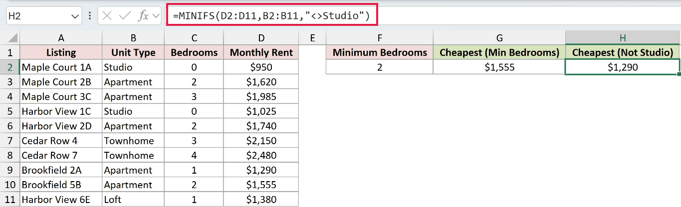
The <> operator means not equal to. Excel excludes Studio rows and returns $1,290 in H2.
Finally, we want the cheapest listing whose name begins with Maple Court.
Here is the formula:
=MINIFS(D2:D11,A2:A11,"Maple Court*")
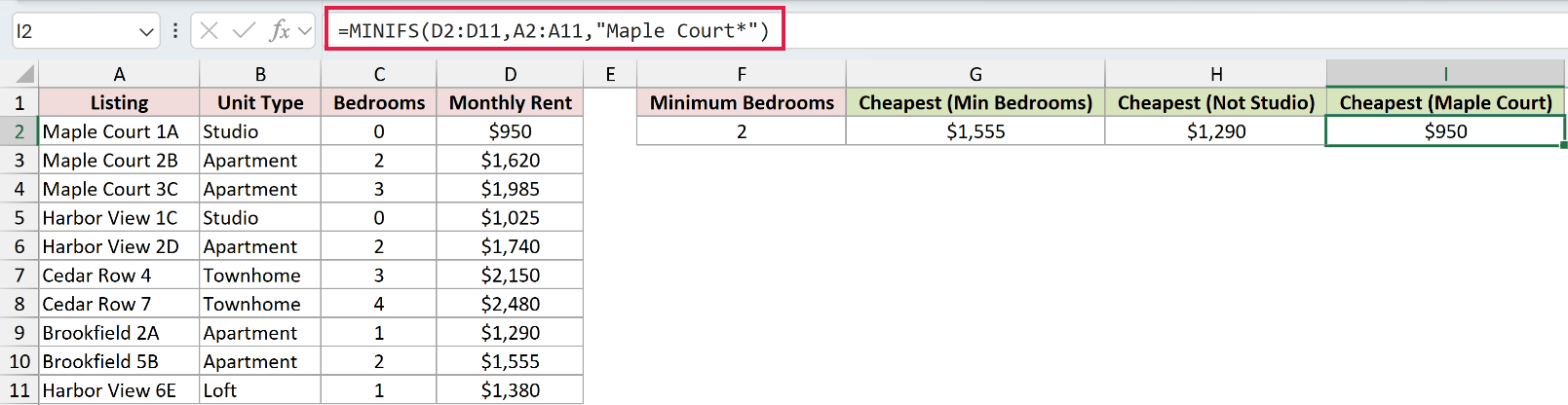
The asterisk matches any text after Maple Court. That includes all three Maple Court listings, and I2 returns $950.
Pro Tip: Use * for any sequence of characters and ? for one character. Add ~ before either symbol when you need to match it literally.
Example 4: Use MINIFS to Ignore Zeros
Consider a coffee cart that records closed days as zero.
Below is the dataset. Columns A through C contain each date, cups sold, and whether the coffee cart was open.
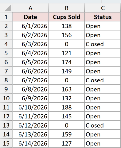
First, we want to see what a plain MIN calculation returns.
Here is the formula:
=MIN(B2:B15)
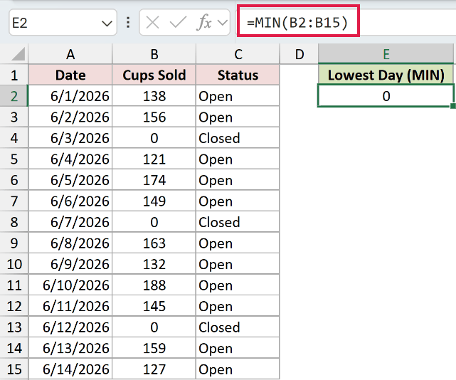
The result in E2 is 0 because closed days are recorded as zero. Excel treats those entries as valid numbers.
To exclude them, we can test the sales range against a greater-than-zero condition.
Here is the formula:
=MINIFS(B2:B15,B2:B15,">0")
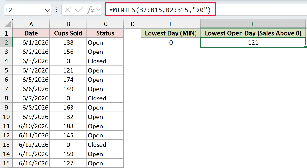
The same range serves as both the minimum range and the criteria range. F2 returns 121, the lowest value above zero.
If the table has a status column, we can use that instead.
Here is the formula:
=MINIFS(B2:B15,C2:C15,"Open")
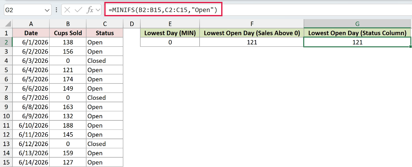
This version includes only rows marked Open and returns 121 in G2. MINIFS ignores blank cells in the minimum range, but it does not ignore zeros.
Example 5: MINIFS Between Two Dates
Next, we’ll find the lowest price inside a date window and handle a missing match properly.
Below is the dataset. Columns A through C hold the price log. Columns E through G state each station and its own start and end dates.
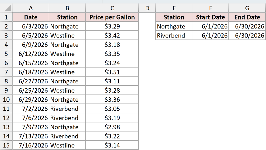
We want each station’s lowest price between the dates shown on its row.
Enter this formula in H2 and copy it down through H3:
=MINIFS($C$2:$C$15,$B$2:$B$15,E2,$A$2:$A$15,">="&F2,$A$2:$A$15,"<="&G2)
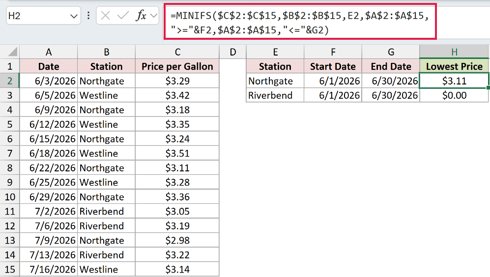
The data ranges stay absolute, while E2, F2, and G2 change with each row. That lets every station use its own date window.
Northgate returns $3.11 in H2. Riverbend has no prices from 6/1/2026 through 6/30/2026, so H3 returns $0.00.
That zero isn’t an error, so IFERROR cannot catch it. COUNTIFS must check whether any rows match before MINIFS runs.
Enter this guarded formula in I2 and copy it down through I3:
=IF(COUNTIFS($B$2:$B$15,E2,$A$2:$A$15,">="&F2,$A$2:$A$15,"<="&G2)=0,"No prices in range",MINIFS($C$2:$C$15,$B$2:$B$15,E2,$A$2:$A$15,">="&F2,$A$2:$A$15,"<="&G2))
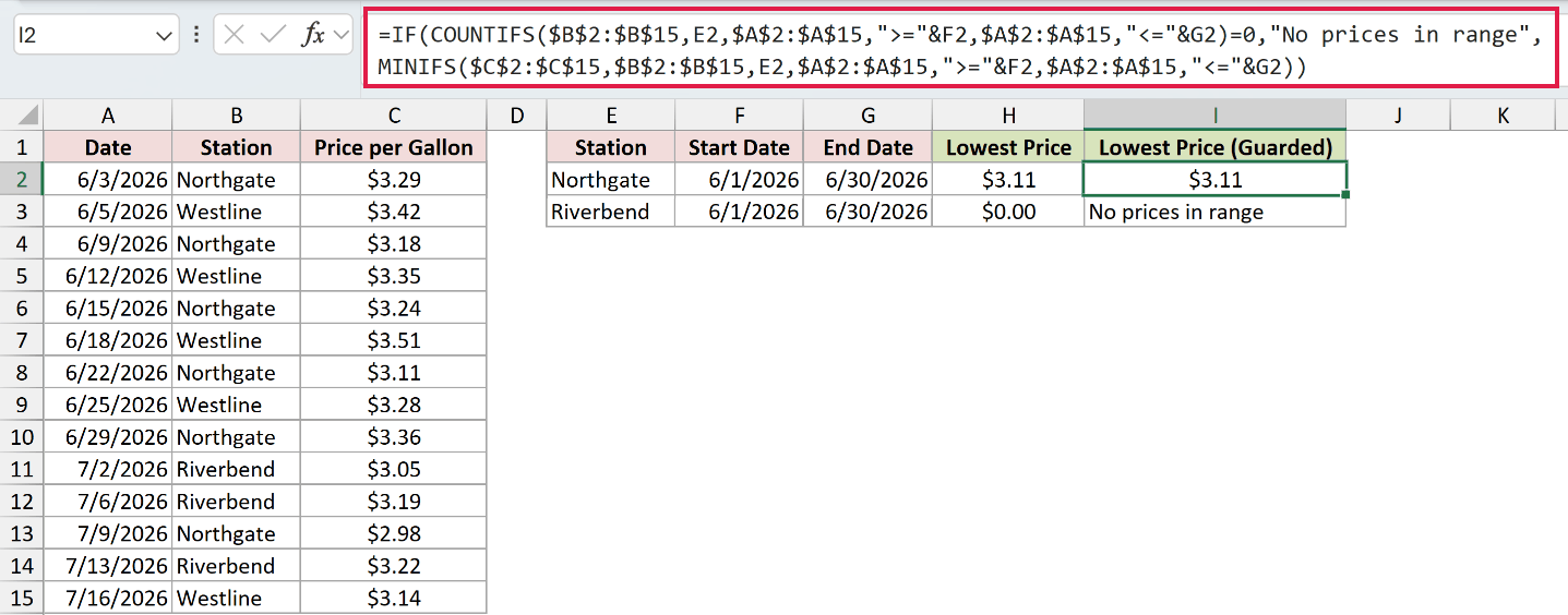
I2 still returns $3.11 for Northgate. I3 shows “No prices in range” for Riverbend instead of a believable-looking $0.00.
In Excel 2021 and later, MIN with FILTER is often safer for this job because no matching rows produce #CALC! instead of zero.
Example 6: MINIFS for Each Unique Group
Finally, let’s calculate a lowest bid for every project with spilled formulas.
Below is the dataset. Columns A through C contain project names, contractors, and bid amounts.
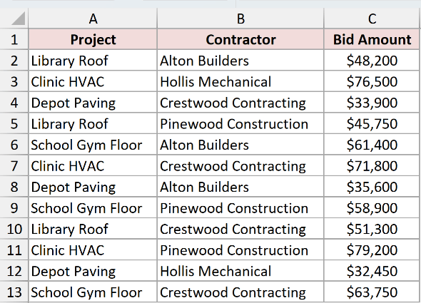
We want a unique project list first, followed by the lowest bid for every project.
Here is the UNIQUE formula:
=UNIQUE(A2:A13)
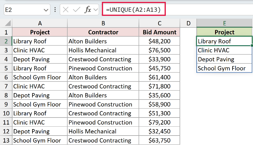
The formula in E2 spills Library Roof, Clinic HVAC, Depot Paving, and School Gym Floor into E2:E5.
Now we can pass that spilled list to MINIFS as the criteria argument.
Here is the MINIFS formula:
=MINIFS(C2:C13,A2:A13,E2:E5)
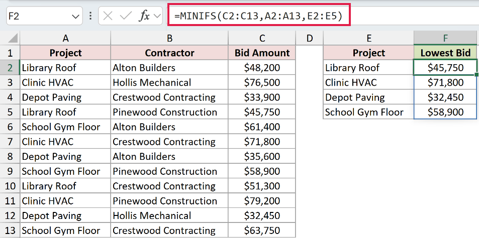
The formula spills four results into F2:F5. They are $45,750, $71,800, $32,450, and $58,900 in the same project order.
MINIFS accepts the array in its criteria argument. Its minimum range and criteria range still point to real worksheet cells.
In Microsoft 365, GROUPBY can return the project names and minimum bids as one spilled table when you don’t need the separate UNIQUE list.
Tips & Common Mistakes
- MINIFS is available in Excel 2019, Excel 2021, Excel 2024, and Microsoft 365. Excel 2016 and earlier return #NAME?.
- In Excel 2016 and earlier, use an array formula such as
=MIN(IF(criteria_range=criteria,min_range))and confirm it with Ctrl+Shift+Enter. - The minimum range and every criteria range must be real worksheet ranges. MINIFS rejects array constants in those arguments.
- The minimum range and criteria ranges must have the same size and shape. Mismatched ranges return #VALUE!.
- Comparison operators joined to cell references need an ampersand, as in
">="&F2. Writing">=F2"treats F2 as text. - Text criteria are not case-sensitive. The criteria
"open"and"Open"match the same rows. - MINIFS returns 0 when nothing matches. Use COUNTIFS as a guard because IFERROR does not react to a valid zero.
- A zero in the minimum range is a real value and can become the result. Blank cells are ignored.
- When the minimum range contains dates, format the result cell as a date or Excel displays the underlying serial number.
- MINIFS returns a value, not the rest of its row. Pair the result with XLOOKUP or INDEX and MATCH when you need related details.
MINIFS can find minimum values using one or several conditions, including operators, wildcards, dates, and criteria from a spilled list.
Keep the ranges the same size, and remember that MINIFS returns zero when no rows match.
Related Excel Functions / Articles:
Other Excel articles you may also like:
