AGGREGATE Function in Excel

AGGREGATE lets you calculate a clean result from a messy range without editing the source data.

You’ll see six practical ways to use it, from simple summaries to matching records.

AGGREGATE returns a single value, but it also works inside dynamic array formulas that can spill several results.

AGGREGATE Function Syntax in Excel

AGGREGATE uses a function number, an options number, and one or more references to decide what to calculate and what to ignore.

=AGGREGATE(function_num, options, ref1, [ref2], ...)

For function numbers 14 through 19, Excel uses the array form:

=AGGREGATE(function_num, options, array, [k])

• function_num is a number from 1 to 19 that selects the calculation. For example, 1 means AVERAGE, 9 means SUM, 14 means LARGE, and 15 means SMALL.
• options is a number from 0 to 7 that controls what Excel ignores. Omitting it behaves as option 0, which ignores nested SUBTOTAL and AGGREGATE results only.
• ref1 is the first reference or range to evaluate.
• [ref2] represents any additional references. You can supply up to 253 references for calculations that accept them.
• For function numbers 14 through 19, the arguments are named array and [k]. The k value identifies a rank, percentile, or quartile.

When to Use AGGREGATE Function

• Calculate an average, sum, maximum, or other summary while ignoring error values.
• Total only visible rows after filtering a list or manually hiding rows.
• Build a grand total that excludes nested SUBTOTAL and AGGREGATE results.
• Find ranked or conditional values without adding helper columns.
• Extract the first, second, or later matching record in older Excel versions.

Example 1: Average While Ignoring Errors

Start with a range containing a couple of calculation errors.

Below is the dataset of kiosk locations, weekly sales, transactions, and average ticket values. Locations with zero transactions produce #DIV/0! in the Avg Ticket column.

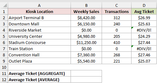
I want to average the valid ticket values without changing or removing the error cells.

Here is the formula:

=AGGREGATE(1,6,D2:D9)

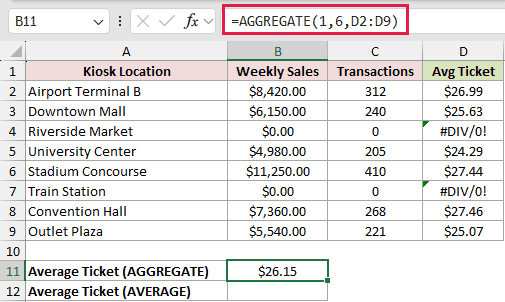
For comparison, here is the regular AVERAGE formula:

=AVERAGE(D2:D9)

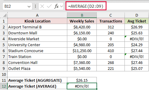
The 1 tells AGGREGATE to calculate an average. Option 6 tells it to ignore error values in the supplied range.

The valid ticket values average $26.15. The regular AVERAGE formula returns #DIV/0! because D4 and D7 contain errors.

Pro Tip: Option 6 ignores errors in the referenced range. It does not repair the underlying division errors, so check whether those errors represent missing data or a genuine problem.

Example 2: Total Visible Filtered Rows

Filtered lists are where AGGREGATE can be especially handy.

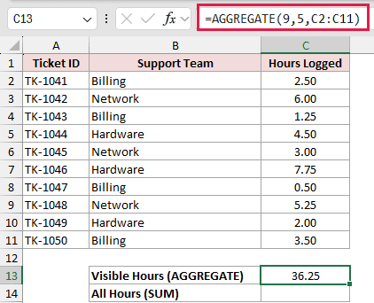
Below is the dataset of support tickets, assigned teams, and hours logged for each ticket.

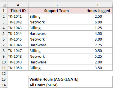
I want the total hours to change when I filter or hide rows.

Here is the formula:

=AGGREGATE(9,5,C2:C11)

And here is the plain SUM formula for comparison:

=SUM(C2:C11)

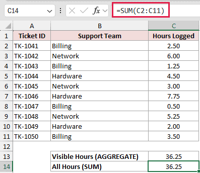
Function number 9 selects SUM. Option 5 tells AGGREGATE to ignore hidden rows while keeping error values and nested totals in scope.

With every row visible, both formulas return 36.25 hours. After filtering Support Team to Billing, AGGREGATE returns 7.75 hours while SUM remains 36.25.

Here is how those totals look after applying the Billing filter.

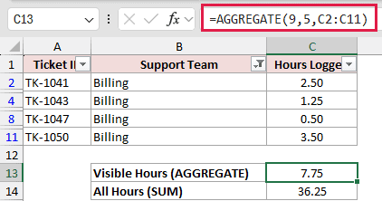
Pro Tip: Only the odd options, 1, 3, 5, and 7, skip hidden and filtered rows. The even options, 0, 2, 4, and 6, count every row.

Example 3: Skip Nested Subtotals

Regional subtotals can make a plain SUM count the same values twice.

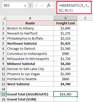
Below is the dataset of freight routes and costs, with an AGGREGATE subtotal after each regional group.

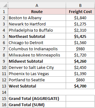
I want one grand total that adds the route costs but skips the three subtotal rows.

Here is the formula:

=AGGREGATE(9,3,B2:B13)

And here is the plain SUM formula for comparison:

=SUM(B2:B13)

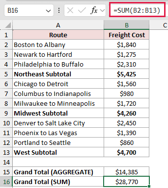
Option 3 ignores hidden rows, error values, and nested SUBTOTAL or AGGREGATE results. The grand total is $14,385.

SUM includes the original freight costs and the three regional subtotals. That double-counting produces $28,770, exactly twice the correct total.

Pro Tip: Options 0 through 3 ignore nested SUBTOTAL and AGGREGATE formulas. Options 4 through 7 do not, so choose the options number carefully.

Example 4: Spill Top and Bottom Three

AGGREGATE can also return several ranked values at once.

Below is the dataset of insurance agents and policies sold, plus rank numbers 1 through 3 for the two result columns.

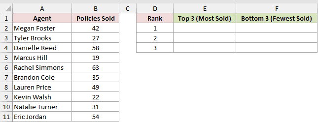
I want the three highest and three lowest policy counts to spill into separate result columns.

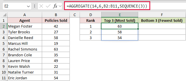
Here is the formula for the top three values:

=AGGREGATE(14,6,B2:B11,SEQUENCE(3))

And here is the formula for the bottom three values:

=AGGREGATE(15,6,B2:B11,SEQUENCE(3))

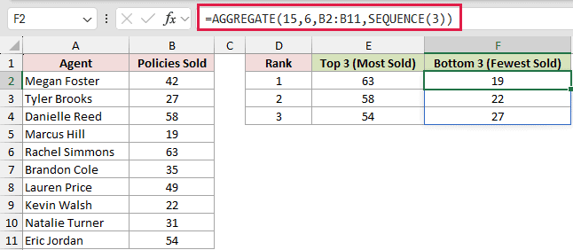
Function number 14 selects LARGE, while 15 selects SMALL. Option 6 ignores errors in the source array.

SEQUENCE supplies the k values 1, 2, and 3. The first formula spills 63, 58, and 54, while the second spills 19, 22, and 27.

In Excel 365, =LARGE(B2:B11,SEQUENCE(3)) and =SMALL(B2:B11,SEQUENCE(3)) are shorter. The AGGREGATE versions still matter when the source may contain errors.

Pro Tip: A blocked spill range causes a #SPILL! error. Clear any values from E3:E4 or F3:F4 so Excel has room for all three results.

Example 5: Find the Largest Value by Category

This next calculation finds a category result without a helper column.

Below is the dataset of job IDs, trades, and job values. A small criteria area lists the four trades beside the result column.

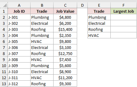
I want to return the largest job value for the trade named in E2.

Here is the formula:

=AGGREGATE(14,6,$C$2:$C$13/($B$2:$B$13=E2),1)

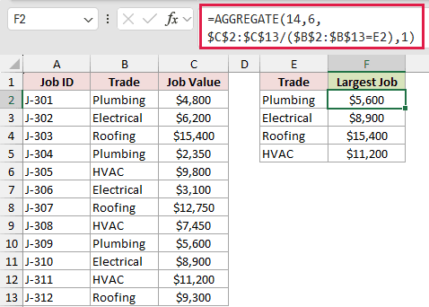
The test $B$2:$B$13=E2 returns TRUE for Plumbing and FALSE for every other trade.

Dividing by TRUE keeps matching values. Dividing by FALSE creates errors, which option 6 ignores. Function number 14 with k set to 1 returns the largest match.

The copied formulas return $5,600 for Plumbing, $8,900 for Electrical, $15,400 for Roofing, and $11,200 for HVAC.

In Excel 2019 and later, =MAXIFS(C2:C13,B2:B13,E2) is more direct. The AGGREGATE form still works in Excel 2010 and can ignore source errors.

Example 6: Pull the Nth Matching Record

The last example uses AGGREGATE to pull matching records in order.

Below is the dataset of invoice numbers, clients, and payment statuses. The Match # column requests the first through fourth overdue clients.

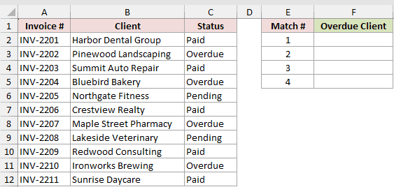
I want to return each overdue client in the order the records appear.

Here is the formula:

=INDEX($B$2:$B$12,AGGREGATE(15,6,(ROW($B$2:$B$12)-ROW($B$2)+1)/($C$2:$C$12="Overdue"),E2))

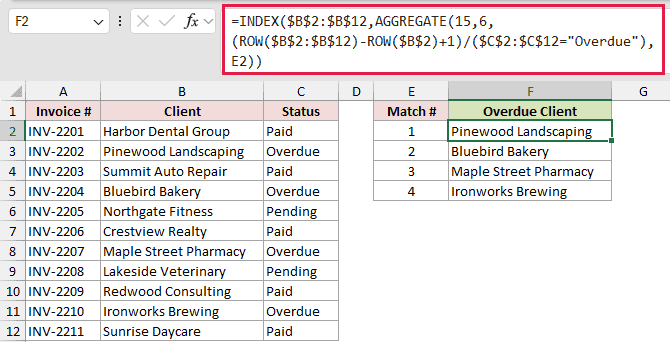
The status test keeps row positions for Overdue invoices and creates errors for other rows. AGGREGATE ignores those errors and returns the requested matching position.

INDEX uses that position to return the client. The four results are Pinewood Landscaping, Bluebird Bakery, Maple Street Pharmacy, and Ironworks Brewing.

In Excel 365, =FILTER(B2:B12,C2:C12="Overdue") returns all four names with a shorter spilling formula.

The AGGREGATE pattern still works in older Excel versions and supports nth-match requests.

Tips & Common Mistakes

• AGGREGATE is available in Excel 2010 and later. Dynamic array helpers such as SEQUENCE and FILTER require a newer Excel version.
• Check both control numbers. The first selects the calculation, while the second decides which rows, errors, and nested results Excel ignores.
• Function numbers 14 through 19 need a k argument. Leaving it out returns #VALUE! because Excel does not know which ranked value to return.
• Use vertical ranges. AGGREGATE is designed for vertical references, and 3-D references return #VALUE!.
• Hidden rows, nested SUBTOTAL results, and nested AGGREGATE results are not ignored when the array argument contains a calculation. In Examples 5 and 6, hiding or filtering rows does not change the result because the array is calculated, not a direct reference.
• Options 4 through 7 include nested SUBTOTAL and AGGREGATE results. Use options 0 through 3 when you need a grand total that skips them.

AGGREGATE is most useful when the source data is messy or changes with filtering.

Once you understand its two control numbers, you can adapt one function to many jobs without adding helper columns.

List of All Excel Functions

Related Excel Functions / Articles:

• GROUPBY Function in Excel
• MAX Function in Excel
• How to Sum a Column in Excel?