If you want to convert text to all capital letters in Excel, the UPPER function is the simplest way to do it.
Hand it a string, a code, or a whole column of text, and you get the same text back in uppercase.
In Excel 365, you can also feed UPPER an entire range and the results will spill into the cells below the formula. So one formula uppercases a whole column, no fill handle needed.
In this article, I’ll walk through how UPPER works, how to combine it with TRIM for cleanup, how to use it for case-insensitive comparisons, how to replace the original column with the uppercase version, and the gotchas worth knowing.
UPPER Syntax
Here is the syntax of the UPPER function:
=UPPER(text)
- text – The text you want to convert to uppercase. This can be a string in quotes, a single cell reference, a range (in Excel 365), or the result of another formula.
That’s the whole function. One argument in, uppercase text out.
Numbers, punctuation, and spaces inside the text are left untouched. Only lowercase letters get flipped to uppercase.
Now let me show you a few practical examples of how to use this function.
Example 1: Uppercase a Column of Stock Tickers
Let’s start with a simple example.
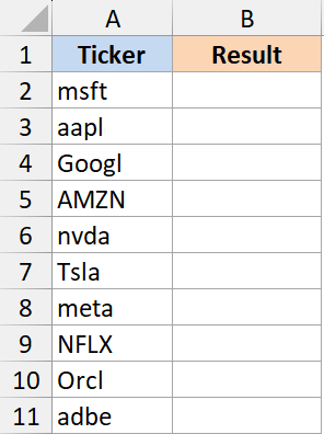
Below is a list of stock tickers pulled from a watchlist. Some are lowercase, some are mixed case, and I want a clean column where every ticker is in uppercase.
Here is the formula:
=UPPER(A2:A11)
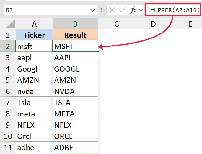
In the above formula, UPPER takes the whole range and converts every lowercase letter to uppercase.
So “msft” becomes “MSFT” and “Googl” becomes “GOOGL”. The result spills into the cells below the formula automatically. No dragging the fill handle, no copy-paste.
If you only need a single value, =UPPER(A2) still works the way it always did. The range form is just the faster way to do a whole column.
Example 2: Clean Up Flight Codes With UPPER and TRIM
Here’s another practical scenario.
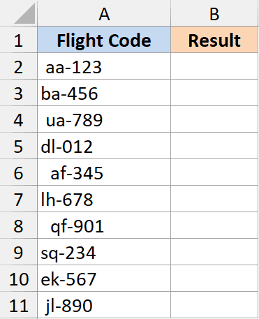
You have a column of flight codes pulled from a booking export. Some were typed lowercase (“aa-123”), some have leading or trailing spaces, and you want them all in the same uniform format.
Here is the formula:
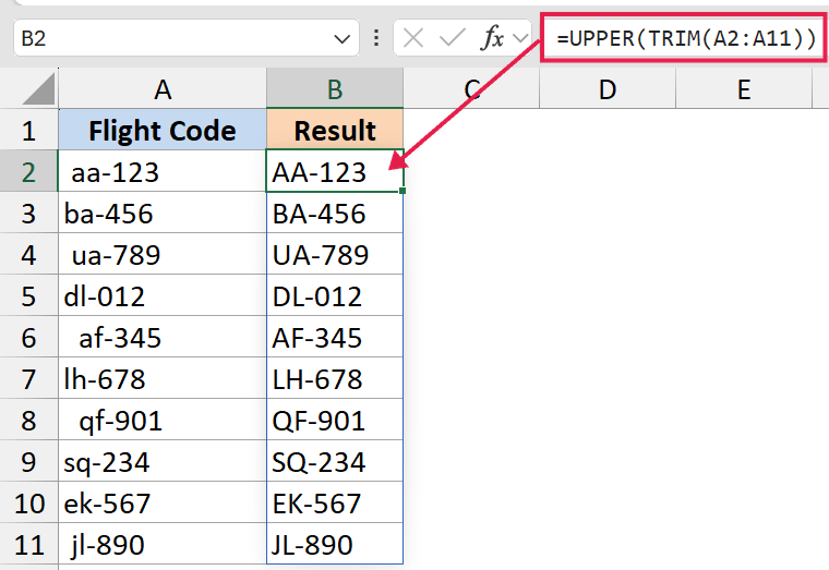
=UPPER(TRIM(A2:A11))
How this formula works:
- TRIM strips leading, trailing, and double spaces from each entry in the range.
- UPPER then converts every lowercase letter in the cleaned text to uppercase.
- The combined result spills down the column in one go.
So ” aa-123 ” becomes “AA-123” and “ba-456 ” becomes “BA-456”. Same pattern works anywhere you want a quick text cleanup before any comparison or lookup.
Wrapping UPPER around TRIM keeps the order right (clean first, then uppercase), but in this case either order produces the same result.
Example 3: Replace the Original Column with Uppercase Values
This one isn’t a formula trick. It’s a workflow people miss when they first start using UPPER.
UPPER returns a new value in a new cell. It does not change the original cell.
So if you want to replace the messy column A with the cleaned uppercase version, you write the spilling formula in a helper column, copy the spilled result, and paste it back as values.
Here’s the workflow:
- In a helper column (say B), enter
=UPPER(A2:A11)in B2. The whole uppercase column spills into B2:B11 automatically. - Select the spilled range B2:B11 and copy it (Ctrl + C).
- Right-click on cell A2, choose Paste Special, then pick Values. Or use the keyboard shortcut Control + Shift + V.
- The original column now holds the uppercase text. Delete the helper column.
The reason Paste Special > Values matters: a regular paste would copy the formula, and the formula points to cells you’re about to overwrite, so you’d end up with a circular reference or garbage.
Pasting as values strips the formula and just keeps the uppercase text.
This is the standard way to “set” the result of any text function in Excel, not just UPPER. Same pattern works for LOWER, PROPER, TRIM, and so on.
Example 4: UPPER vs LOWER vs PROPER
These three functions are the ones you reach for when text casing is off, so it helps to see them side by side.
All three spill cleanly when given a range in Excel 365, so a single formula like =UPPER(A2:A4) or =PROPER(A2:A4) returns the converted column in one shot.
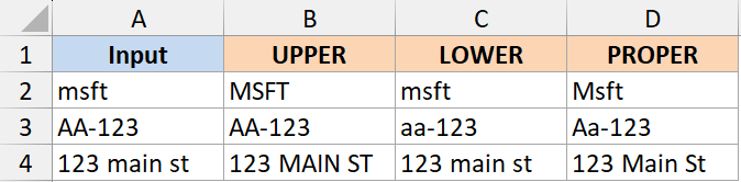
Here’s what each one does to the same input:
| Input | UPPER | LOWER | PROPER |
|---|---|---|---|
| msft | MSFT | msft | Msft |
| AA-123 | AA-123 | aa-123 | Aa-123 |
| 123 main st | 123 MAIN ST | 123 main st | 123 Main St |
Quick guide on when to use which:
- Use UPPER when everything should be in capitals. Stock tickers, country codes, ID numbers, status flags like “ACTIVE” or “PENDING”.
- Use LOWER when everything should be lowercase. Email addresses, URLs, hashtags.
- Use PROPER when you want title case. Names, addresses, city names.
For more on case conversion, see how to change uppercase to lowercase in Excel and how to convert text to sentence case.
Tips & Common Mistakes
- Use the spilling form on a whole range.
=UPPER(A2:A11)returns the entire uppercase column from one formula in 365. There is no need to drag the fill handle for this kind of cleanup anymore. - #SPILL! when something blocks the result. If the cells below your formula already have data, the spilled UPPER won’t have room to land and you get a
#SPILL!error. Clear the spill range and the formula recalculates. - Watch for the
@implicit intersection. Older Excel versions sometimes auto-insert an@symbol when they save a workbook (e.g.=@UPPER(A2:A11)). That collapses the spill to a single cell. Remove the@and the spill comes back. - UPPER returns text in a new cell, not in the source. If you want to replace the original column, follow the Paste Special > Values workflow from Example 4.
- Numbers and special characters are left alone. UPPER only flips lowercase letters to uppercase. Digits, dashes, slashes, and punctuation pass through untouched.
- Whitespace is not removed. UPPER doesn’t trim leading or trailing spaces, and it doesn’t collapse double spaces. If your text has extra whitespace, wrap UPPER with TRIM as in Example 2.
- Accented characters are preserved. “café” becomes “CAFÉ”, not “CAFE”. If you also need to strip accents, you’ll need a separate SUBSTITUTE chain or a helper function.
- Empty cells return empty. If A2 is blank,
=UPPER(A2)returns an empty string, not an error. You don’t need IFERROR around it for empty rows. - It works on numbers stored as text, but not on real numbers. A cell with “abc123” returns “ABC123”. A cell with the number 123 returns “123” (UPPER converts it to text in the process).
- Don’t reach for UPPER just to compare two cells. Plain
=A2=B2is already case-insensitive in Excel. UPPER is only needed when you’re inside EXACT, or building case-sensitive logic that you want to flip to case-insensitive.
That covers the UPPER function and the few quirks worth knowing. In Excel 365 the spilling form turns a column cleanup into a single formula, so most of the time you write =UPPER(A2:A11) once and you’re done. Keep LOWER and PROPER in your back pocket too, since the right pick depends on whether you want all caps, all lowercase, or title case.
Related Excel Functions / Articles: