How to Change Uppercase to Lowercase in Excel

Often when working with text data such as names or address, you will get the data in uppercase, and you may need to convert it into lowercase or propercase.

With my work, I often get all uppercase data from databases or website downloads.

Thanks to Excel, converting uppercase to lowercase (or vice versa) is really easy. All you need to know is the right formula or functionality.

In this tutorial, I will show you three different ways how to change uppercase to lowercase in Excel.

Change Uppercase to Lowercase Using the LOWER function

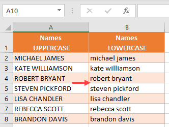
Let’s say that you have a list of names in column A in uppercase, and want to convert them to lowercase in column B.

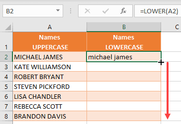
1. In cell B2, enter the below formula. The LOWER function takes a text (or a cell reference) and converts all characters to lowercase.

=LOWER(A2)

2. Position a cursor in the right lower corner of cell B2, until the black cross appears (it’s called the Fill Handle). Drag it until the last populated row (B8).

As a result, you get all the values from column A, changed to lowercase in column B.

Note that as of now, the lowercase result is linked to the uppercase names in column A. So if you make any changes in column A, it would instantly be updated and shown in lowercase in column B.

This also means that you can not delete Column A.

In case you only want to only keep the lowercase value and delete the uppercase data, first convert the formula result in column B into static values.

Just like we converted upper case text to lowercase, you can also do the reverse. You can use the UPPER formula to do that.

Also read: How to Generate Random Letters in Excel?

Change Uppercase to Proper Case Using the PROPER Function

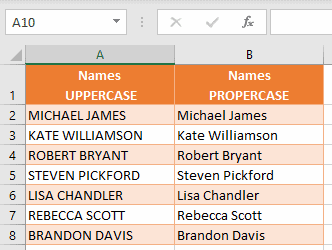
Similar to changing text to lowercase, you can also change a text to a proper case. This means that the changed text will have every first letter of the text capitalized.

So for names, the first character of the first and last name would be in upper case and rest would be in lower case.

Let’s say that you have the same list of names in column A.

When you changed it to lowercase, you probably wanted to have every first letter capitalized, as you’re dealing with names.

1. In cell B2, enter the formula:

=PROPER(A2)

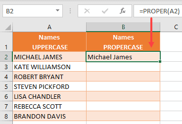
The PROPER function takes a text and converts the first letter of every word in a text to capital letter.

2. Position a cursor in the right lower corner of cell B2, until the black cross appears, and drag it until the last populated row (B8).

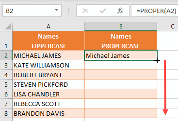
Now, you have the list of names converted from uppercase to proper case.

Again, if you want to delete the names in uppercase and only keep the ones in lowercase, you first need to convert the formulas to values in column B.

Also read: How to Convert to Sentence Case in Excel?

Convert Uppercase to Lowercase Using the Flash Fill

While the formula method is quite easy and straightforward, there is another equally easy and convenient way to change the case of text in Excel.

And that is by using the Flash Fill

Flash Fill is relatively new functionality in Excel that recognizes the pattern and fills cells automatically for you. 

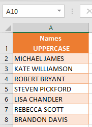
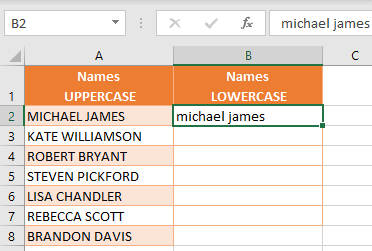
Suppose you have the following list of names in column A, and you want to convert them to lowercase.

Let’s see how to do this using Flash Fill:

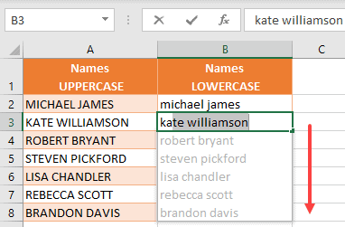
1. In cell B2, enter the value from A2, but in lowercase (“michael james”). The idea here is to enter the expected result so that Excel can deduce what we are trying to do

2. Hit the Enter key to go to cell B3
3. In cell B3, start entering the expected result value from A3, also in lowercase. While you’re typing, Excel recognizes the pattern based on these two cells and recommends populating the rest of the cells (until B8) automatically.

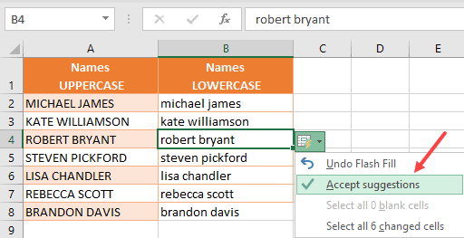
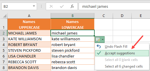
3. If you think Excel has correctly identified the pattern, just hit the Enter key and Excel will automatically fill the cells with the lowercase name. After that, you can see that the Flash Fill icon appears on the right, and you need to click ‘Accept suggestions’ to confirm the values.

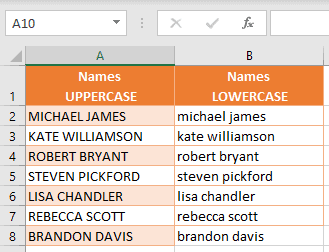
As a final result, you get all names from column B converted to lowercase.

I absolutely love this method as it’s fast, and the resulting values are static. This means that I don’t have to convert these to values (as I had to when I was using the formula).

Note that Flash Fill can work with many different types of data as long as it can identify the pattern. In simple stuff such as changing the case of the text, Flash Fill works flawlessly.

I recommend you still double-check the result of Flash Fill. In some rare cases, it may give a wrong result in case the pattern it identifies is incorrect or only partially correct.

And just the way we used Flash Fill to convert Uppercase to Lowercase, you can also do other text transformations as well, such as converting data to uppercase or proper case.

Using the Flash Fill in the Ribbon

I some cases, it may happen that you don’t see the Flash Fill suggestions while you are typing (where it fill the entire range with expected result in light gray color). If that happens, you can use the below method.

Suppose you have the below dataset in column A that you want to convert to lowercase

1. In cell B2, enter the value from A2, but in lowercase (“michael james”)

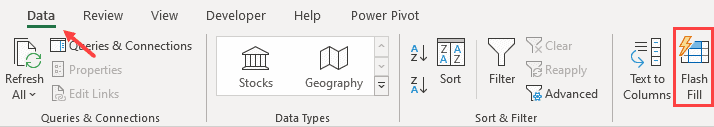
2. In the Ribbon, go to the Data tab, and choose Flash Fill in the Data Tools group.

3. Now you get all values suggestions, and you need to click on the Flash Fill icon to accept values and populate cells.

The final output is the same as in the previous section – you converted all names from column A to lowercase in column B.

In case Excel is not able to identify the pattern with a single input in cell B2, enter the expected result in another cell (B3) and then do the above steps.

Convert Uppercase to Lowercase Using the Power Query

Another option for converting to lowercase is to use the Power Query. This tool is very useful for you if you need to transform your data.

Note: To use Power Query, you should convert your data into an Excel Table. You can do that by selecting any cell in the data and using the keyboard shortcut Control + T (or Command + T if using Mac)

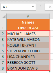
Let’s start from the following data list in column A.

1. Select a range that you want to convert to lowercase (A2:A8).

2. In the Ribbon, go to the Data tab, and choose From Table/Range in the Get & Transform Data group. This option opens the Power Query editor.

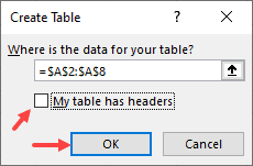
3. In the Create Table dialog box, uncheck the ‘My table has headers’ option, as you selected the data without header and click OK. 

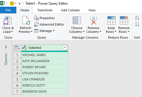
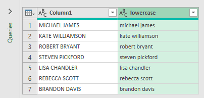
4. Now the Power Query editor is open. As you can see, our data range is imported as column 1. Here, you can see different tabs and options for transforming data.

5. In the Ribbon, go to the Add Column tab, click on the Format icon, and choose lowercase.

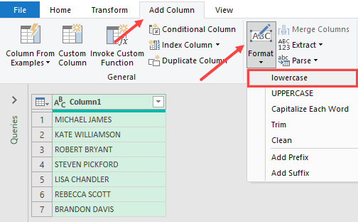
6. This option creates a new column, and populates all rows with values from the original column in lowercase.

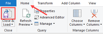
7. Finally, in the Ribbon, go to the Home tab, and choose Close & Load in the Close group. This will close the power query editor and load the table in the new sheet in your Excel file.

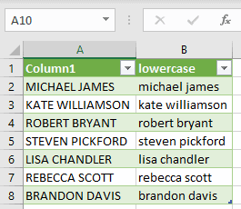
As you can see in the picture below, now you have the new table in the new sheet, with values converted in lowercase.

While I have shown you how to use Power Query to change the names to lower case and keep both the original data and the lowercase data, you can also choose the delete the upper case data and only keep the lowercase one.

One amazing thing about Power Query is that in case your original data changes (more names are added or modified), you don’t need to follow the entire process again.

All you need to do is go to the resulting table (the one with lowercase data), right-click and then click on Refresh. This will automatically check the original data and update the resulting data.

And again, the way we have converted uppercase data to lowercase, you can also do the same to convert data to uppercase or proper case.

So these are three simple ways you can use to convert Uppercase to Lowercase or Proper Case.

I hope you found this tutorial useful.

Other Excel tutorials you may also find useful:

• How to Copy Formatting In Excel
• How to Add Text to the Beginning or End of all Cells in Excel
• How to Remove Text after a Specific Character in Excel
• How to Count How Many Times a Word Appears in Excel (Easy Formulas)
• How to Reverse a Text String in Excel (Using Formula & VBA)
• How to Merge First and Last Name in Excel
• How to Change All Caps to Lowercase Except the First Letter in Excel?