Make Pivot Table from Multiple Sheets

You want to create a Pivot Table from data spread across multiple sheets in a workbook. How do you do it? 

In this tutorial, I will show you three ways to create a Pivot Table from multiple sheets:  

1. Use Power Query to append datasets and create a Pivot Table– Combine multiple datasets with the same column structure into one and create a Pivot Table from the appended data.  
2. Use Power Query to merge datasets and build a Pivot Table – Merge multiple datasets with different column structures but common keys into a single table and build a Pivot Table from the merged data.  
3. Use Power Pivot – Create a Pivot Table by linking multiple datasets with different column structures but common keys in the Power Pivot Data Model.

Method #1: Append Datasets and Create Pivot Table from the Appended Datasets

If you have datasets with the same column structure in multiple sheets, you can use Power Query to append them into a single table and then create a Pivot Table from that table.

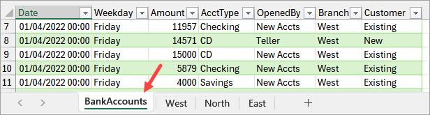
Suppose you have three tables with the same column structure in three worksheets: West, North, and East.

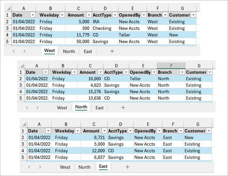
Each table contains information about new accounts opened by new and existing customers in a specific bank branch. 

You want to create a Pivot Table from the multiple tables summarizing the amount of new deposits, broken down by branch and account type.

You can use the steps below to append the three tables into one in Power Query and create the desired Pivot Table based on the combined table.

Step #1: Use Power Query to Append the Multiple Datasets into One

Follow the steps below to combine the datasets in Power Query.

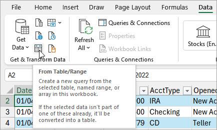
1. Select any cell in the table on the ‘West’ worksheet.

Note: If your dataset is not a table, convert it to one by selecting any cell in the dataset and pressing CTRL + T.

2. Open the Data tab and click the From Table/Range command button on the Get & Transform Data group.

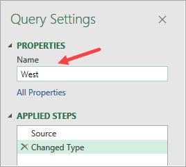
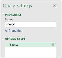
The above step loads the table data onto the Power Query Editor. By default, the query inherits the name of the source table. 

You can rename the query in the Name box on the Query Settings panel on the right. In this example, I have renamed it ‘West.’

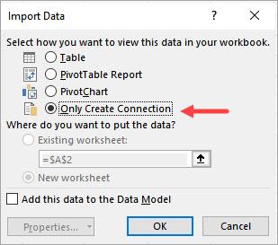
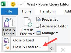
3. On the Home tab, click the bottom part of the Close & Load command button and select the ‘Close & Load To’ option.

The above step opens the Import Data dialog box.

4. On the Import Data dialog box, select the ‘Only Create Connection’ option and click OK.

5. Repeat steps 1 to 4 for the data in the other worksheets.

When you are done, all the queries will be listed in the Queries & Connections pane on the right.

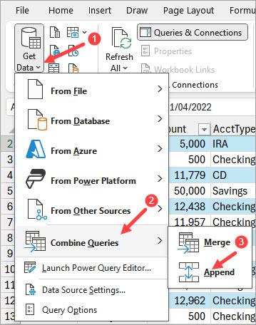
6. On the Data tab, open the Get Data drop-down list on the Get & Transform Data group, hover over the Combine Queries option, and click the Append option on the submenu.

The above step opens the Append feature.

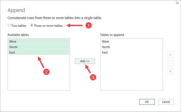
7. On the Append feature, do the following:

• Select the ‘Three or more tables’ option because we want to append three tables.
• Select all the tables on the ‘Available tables’ box on the right (select the first table, press and hold down the Shift key, and select the last table).
• Click the Add button to add the selected tables to the ‘Tables to append’ box on the right.
• Click OK.

The above step loads data from the appended tables into the Power Query Editor as a query named ‘Append1.’

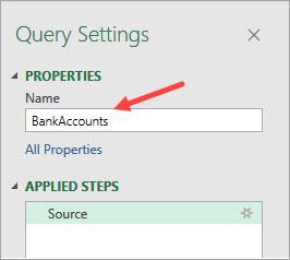
You can rename the query on the Name box on the Query Settings panel on the right. In this example, I have renamed it ‘BankAccounts.’

8. On the Home tab, click the top part of the Close & Load command button. 

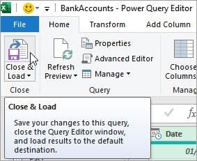
The above step saves changes to the ‘BankAccounts’ query, closes the Power Query Editor window, and loads the appended queries as one table to a new worksheet.

Step #2: Create a Pivot Table

Follow the steps below to make a Pivot Table from the appended datasets:

1. Select any cell in the ‘BankAccounts’ table.
2. On the Insert tab, open the Pivot Table drop-down list on the Tables group.

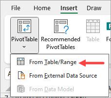
The above step opens the ‘PivotTable from table or range’ dialog box.

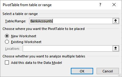
3. Click OK on the ‘PivotTable from table or range’ dialog box to accept the default options.

The above step creates an empty Pivot Table on a new worksheet and displays the Pivot Table Fields task pane on the right of the Excel window.

4. Create your Pivot Table by dragging fields on the left of the task pane between areas on the right. 

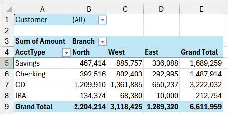
In this example, I have dragged the Customer field to the Filters area, Branch field to the Columns area, AccType field to the Rows area, and the Amount field to the Values area.

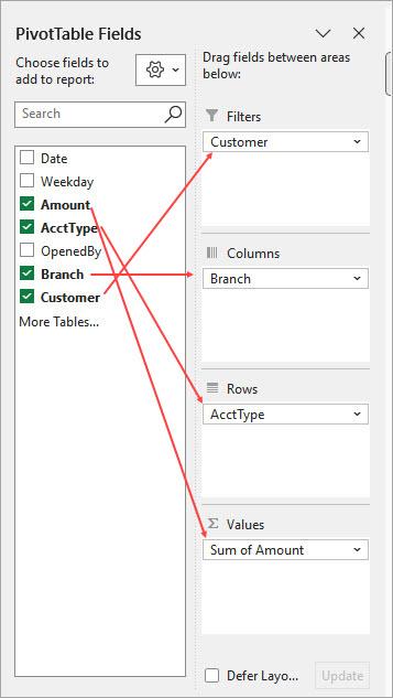
The resultant Pivot Table summarizes the amount of new deposits in North, West, and East bank branches broken down by account type.

Also read: How to Copy a Pivot Table in Excel?

Method #2: Use Power Query to Merge Datasets and Build a Pivot Table from the Merged Datasets

If you have multiple datasets with different column structures and common keys, you can use Power Query to merge them into a single table and then create a Pivot Table from the merged table.

Note: A key is a column or a combination of columns uniquely identifying a table row.

Suppose you have three tables with different column structures and common keys in three worksheets: Customers, InvoiceHeader, and InvoiceDetails.

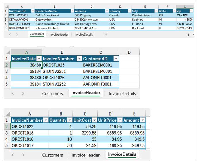
Note: The Customers and InvoiceHeader tables share a common key: CustomerID. The InvoiceHeader and InvoiceDetails tables share a common key: InvoiceNumber.

You want to create a  Pivot Table summarizing the total invoice amounts for each customer in each country.

You can use the steps below to merge the three tables into one in Power Query and create the desired Pivot Table based on the merged table.

Step #1: Use Power Query to Merge the Multiple Datasets into One

Follow the steps below to merge the datasets in Power Query.

1. Load the data of the three tables onto Power Query Editor as explained in Method #1 above. 

Power Query lists the resultant queries on the Queries & Connections task pane on the right of the Excel window.

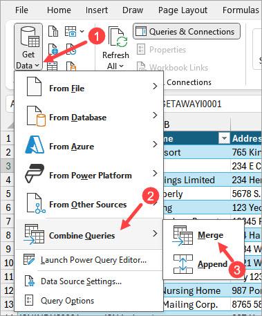
2. On the Data tab, open the Get Data drop-down list on the Get & Transform Data group, hover over the Combine Queries option, and click the Merge option on the submenu.

The above step opens the Merge feature.

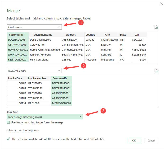
3. On the Merge feature, select the first two tables and matching keys/columns. Choose the ‘Join Kind’ to define how the tables should be joined, then click OK.

In this example, I chose the Customers and InvoiceHeader tables and selected CustomerID as the matching column (click the header of the CustomerID column in both tables). I selected the ‘Inner’ join because I am only interested in customers who have invoices.

Note: Power Query allows merging only two tables at a time. First, I will merge the Customers and InvoiceHeader tables into a query. Then, I will merge this new query with the third table, InvoiceDetails.

The above step creates a  ‘Merge1’ query in Power Query Editor. You can rename the query or leave it as is. I have left it as is.

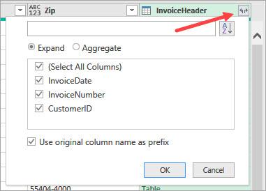
Notice that the columns from the InvoiceHeader table are collapsed in ‘Table’ in the last column of the query. 

3. Click the expand icon in the last column of the query, select the specific columns of the second table to include, and click OK.

4. On the Home tab, click the bottom part of the Close & Transform command button on the Get & Transform Data group and select the ‘Close & Load To’ option.

The above step opens the Import Data dialog box.

5. On the Import Data dialog box, select the ‘Only Create Connection’ option and click OK.

6. On the Data tab, open the Get Data drop-down list on the Get & Transform Data group, hover over the Combine Queries option, and click the Merge option on the submenu.

The step above reopens the Merge feature.

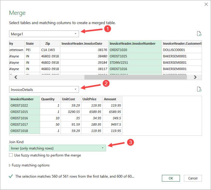
7. On the Merge feature, select the new query, the third table, the ‘Join Kind,’ and click OK.

In this case, I have selected ‘Merge1,’ ‘InvoiceDetails,’ and the ‘Inner’ join.

8. Repeat step 3 above for the new ‘Merge2’ query.
9. On the Home tab, click the top part of the Close & Load command button on the Get & Transform Data group. 

The above step saves changes to the ‘Merge2’ query, closes the Power Query Editor window, and loads the merged queries as a table onto a new worksheet.

Step #2: Create a Pivot Table

Follow the steps in step #2 of Method #1 above to make a Pivot Table from the merged datasets.

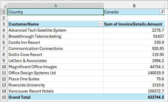
In this example, I have dragged the Country field to the Filters area, the CustomerName field to the Rows area, and the Amount field to the Values area.

The above steps create a Pivot Table showing the invoice amounts for each customer in each country. In this example, the Pivot Table is filtered to show the total invoice amounts for each customer in Canada.

Also read: How to Merge Two Excel Files?

Method #3: Use Power Pivot to Make a Pivot Table from Multiple Sheets

You can use Power Pivot to create a Pivot Table from multiple sheets in a workbook. Power Pivot is part of Excel’s Power Business Intelligence (BI) suite.

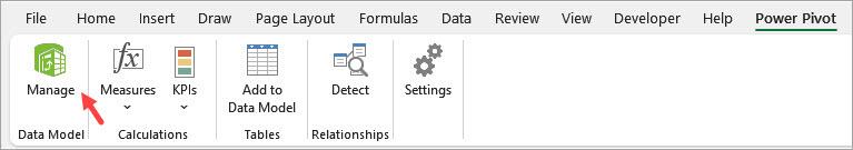
If  the Power Pivot tab is activated , you will see it on the Ribbon.

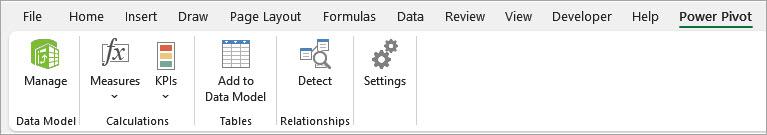
If you do not see the Power Pivot tab on the Ribbon, activate it using the steps below.

Activate Power Pivot tab

1. Click the File button on the Ribbon to open the Backstage view.
2. Click Options on the left panel of the Backstage view.

The above step opens the Excel Options dialog box.

3. On the Excel Options dialog box, select Add-ins category on the left panel, open the Manage drop-down list on the right, choose the COM Add-ins option, and click the Go button.

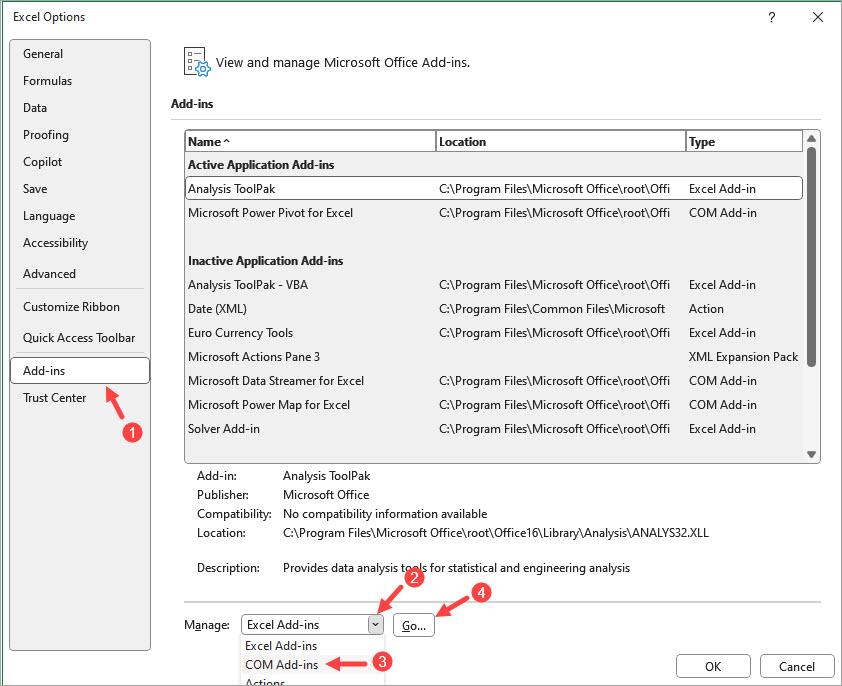
The above step opens the COM Add-ins dialog box

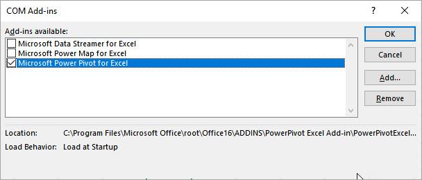
4. On the COM Add-ins dialog box, check the checkbox next to the Microsoft Power Pivot for Excel add-in and click OK.

5. Close and restart Excel.

Make a Pivot Table from Multiple Sheets

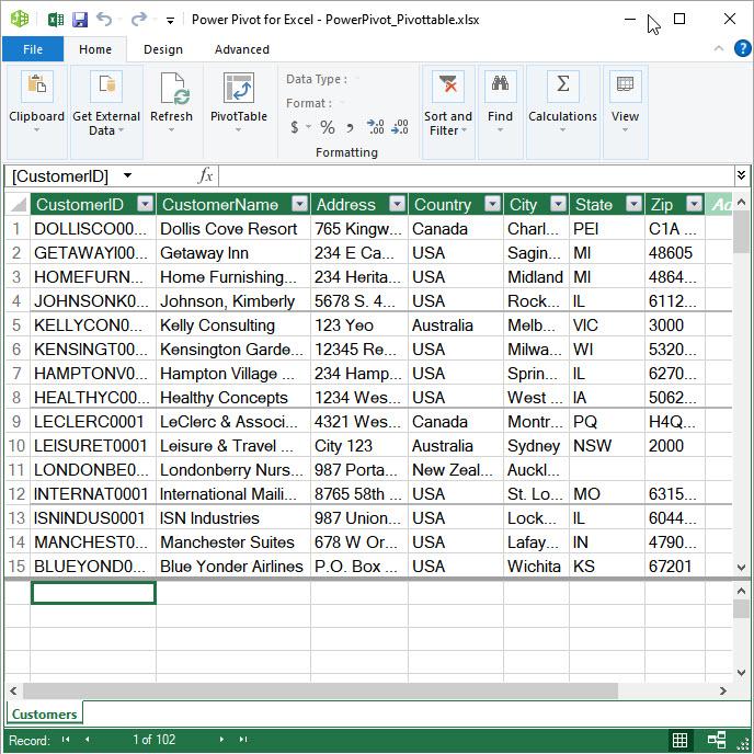
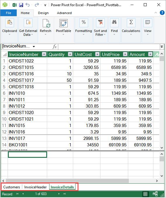
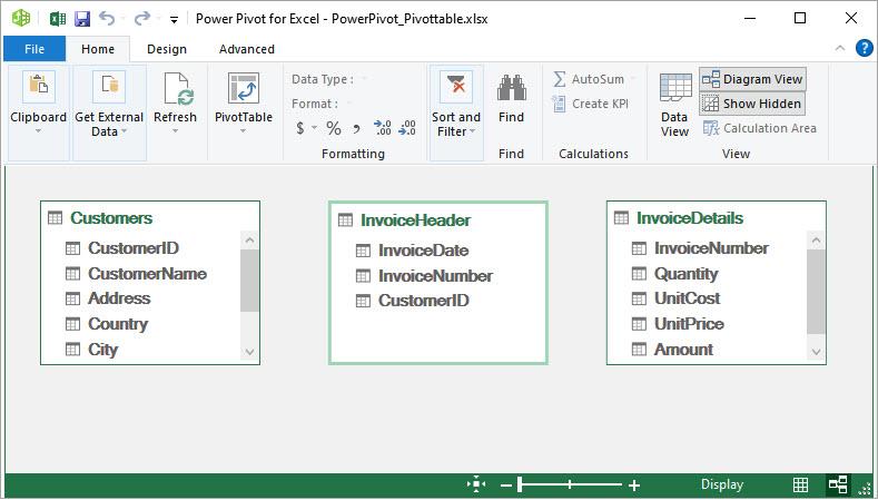
Suppose you have datasets in three worksheets: Customers, InvoiceHeader, and InvoiceDetails.

The Customers dataset contains details such as Customer ID and Customer Name. The Invoice Header dataset links invoices to specific customers, while the Invoice Details dataset provides itemized information for each invoice.

You want to create a  Pivot Table summarizing the total invoice amounts for each customer in each country.

Use the steps below to make the Pivot Table.

Step #1: Give the Tables Meaningful Names

If the datasets are not tables, convert them to tables by pressing CTRL + T.

Give the tables meaningful names rather than the default Table1, Table2, and Table3 by doing the following:

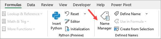
1. Open the Formulas tab and click the Name Manager icon on the Defined Names group.

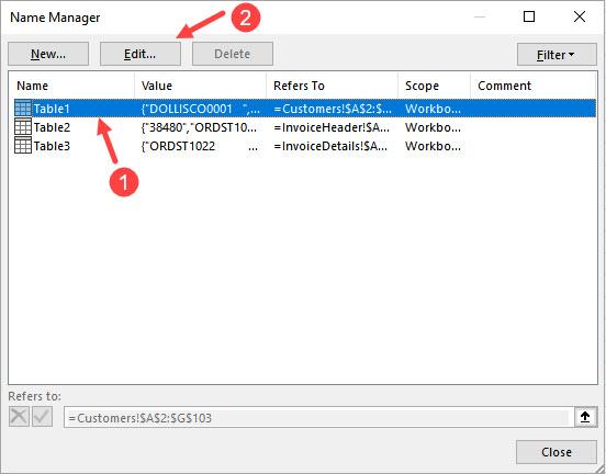
The above step opens the Name Manager feature.

2. On the Name Manager feature, select the first table name, in this case Table1, and click the Edit button.

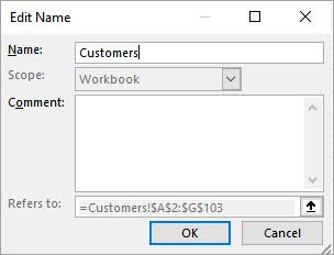
The above step opens the Edit Name feature.

3. Rename the table on the Edit Name feature and click OK.

4. Repeat steps 2 and 3 above to rename the other tables.
5. Close the Name Manager feature.

Step #2: Add the Tables to the Power Pivot Data Model

Use the steps below to add the tables to the Power Pivot data model.

1. Click any cell in the Customers table.
2. On the Power Pivot tab, click the Add to Data Model command button on the Tables group.

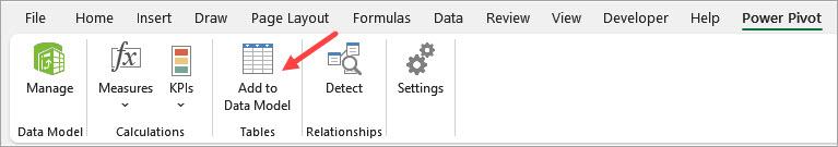
Power Pivot creates a copy of the Customers table and activates the Power Pivot window.

Notice that although the Power Pivot window looks like Excel, it is a separate program. You can switch between Excel and Power Pivot by clicking each respective icon on the taskbar. 

3. Repeat steps 1 and 2 for the other Excel tables.

Each table will be shown on its own tab in Power Pivot.

Step #3: Create Relationships Between the Power Pivot Tables

Up to this point Power Pivot knows that it has three tables in its data model but does not know how the tables relate to each other.

Note: If you accidentally close the Power Pivot window, you can reopen it by clicking the Manage command button on the Power Pivot tab.

You need to link these tables by defining the relationship between them using the steps below.

1. On the Power Pivot Home tab, click the Diagram View command button on the View group.

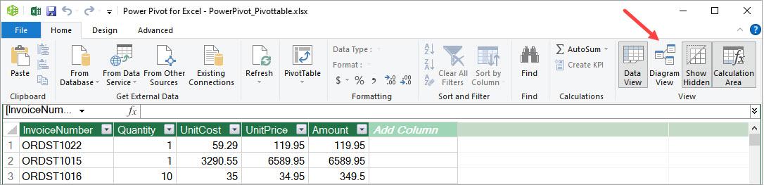
The Diagram View allows you to see all the tables in the Power Pivot data model.

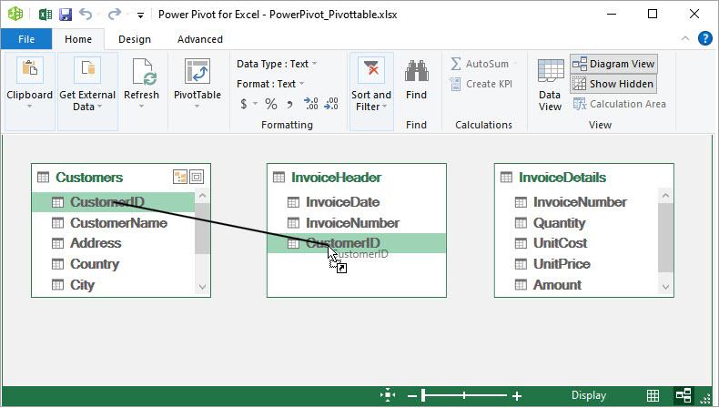
2. Click the CustomerID field in the Customers table, hold down the left mouse button and drag a line to the CustomerID field in the InvoiceHeader table.

3. Click the InvoiceNumber field in the InvoiceHeader table, hold down the left mouse button and drag a line to the InvoiceNumber field in the InvoiceDetails table. 

Power Pivot shows join lines between the tables.

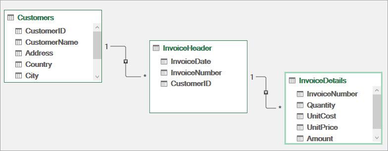
The joins are one-to-many, meaning one customer can have many invoices.

Step #4: Create a Pivot Table

Use the steps below to create the desired Pivot Table.

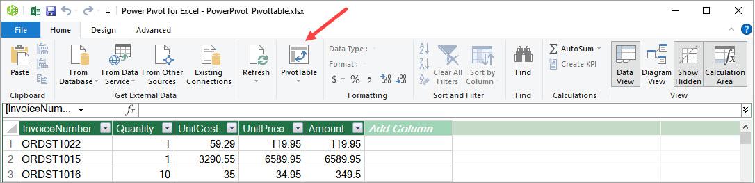
1. Activate the Power Pivot window and click the Pivot Table command button on the Home tab.

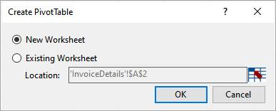
The above step opens the Create Pivot Table dialog box.

2. On the Create PivotTable dialog box, click OK to create the Pivot Table on a new worksheet.

The above step creates an empty Pivot Table on a new worksheet and displays the Pivot Table Fields task pane on the right of the Excel window.

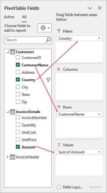
3. Drag the fields on the left of the Pivot Table Fields task pane between the areas to the right of the pane.

In this example, I have dragged the Country field to the Filters area, the CustomerName field to the Rows area, and the Amount field to the Values area.

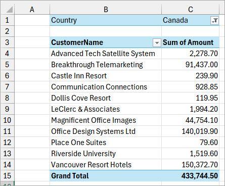
The above steps create a Pivot Table showing the total invoice amounts for each customer in each country. In this example, the Pivot Table is filtered to show the total invoice amounts for each customer in Canada. 

I have shown you three ways to make a PivotTable from multiple sheets. I hope you found the tutorial helpful.

Other articles you may also like:

• How to Move Pivot Table in Excel?
• How to Group by Quarters in Excel Pivot Table?
• Reorder Rows in Pivot Table in Excel
• How to Clear Pivot Table Cache?