How to Reorder Rows in Pivot Table in Excel (4 Easy Ways)

When you create a Pivot Table, by default, Excel orders the rows based on the row labels’ data type.

This means that:

Text labels are arranged alphabetically from A to Z
Dates are ordered chronologically from oldest to newest, and
Numbers are sorted in ascending order from smallest to largest.

If the default row order in a Pivot Table doesn’t meet your needs, you can rearrange the rows as desired.

I’ll show you how to reorder rows in a Pivot Table using drag and drop, Move options, and sorting using Excel’s built-in options and a custom list.

Table of Contents

Method #1: Use Drag and Drop to Reorder Rows in a Pivot Table

You can manually reorder rows in a Pivot Table using drag and drop.

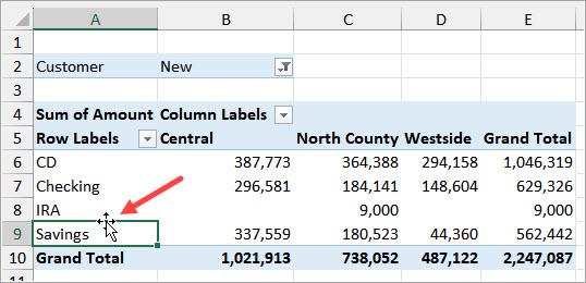
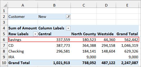
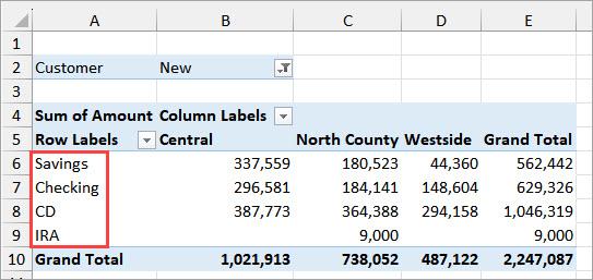
The Pivot Table below shows the total deposits made by new customers at various bank branches, organized in ascending alphabetical order by account type: CD, Checking, IRA, and Savings.

You want to reorder the rows in the Pivot Table so that the ‘Savings’ row appears before the ‘CD’ row.

Here’s how you can do it:

Select the cell containing the ‘Savings’ row label, and hover over the top edge of the cell until you see a four-headed arrow.

Select the row label to move in Pivot Table

Press and hold down the left mouse button and drag the row label to the top edge of the cell containing the ‘CD’ label. Notice the green bar or insertion indicator that appears as you drag.

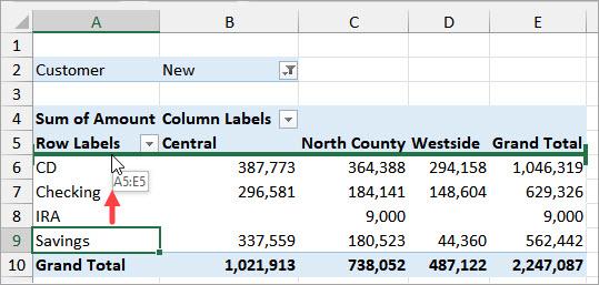
Release the mouse button to drop the ‘Savings’ row at the desired location.

Also read: Move Pivot Table in Excel

Method #2: Use Move Options to Reorder Rows in a Pivot Table

You can reorder rows in a Pivot Table using the ‘Move’ options on the context menu of the row labels.

Suppose you have the Pivot Table below, which displays the total deposits made by new customers at various bank branches. The data is organized alphabetically in ascending order by account type: CD, Checking, IRA, and Savings.

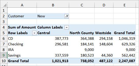
You want to rearrange the rows in the Pivot Table so that the ‘Savings’ row appears before the ‘CD’ row.

Here’s how to do it:

Right-click the cell containing the ‘Savings’ row label, hover over the ‘Move’ option, and click the ‘Move “Savings” to Beginning’ option on the submenu.

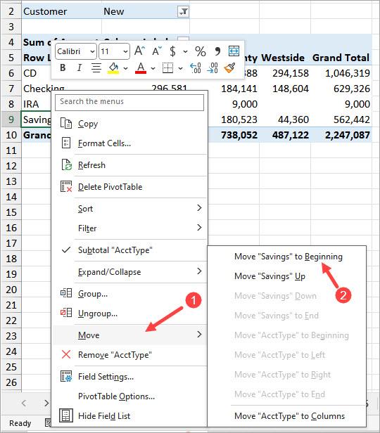
Excel moves the ‘Savings’ row to the beginning of the list of rows.

Explanation of the Move Options

The ‘Move’ option has four sub-options.

Below is the explanation of each option:

Move to Beginning – Moves the selected row label and its row to the beginning of the list.
Move Up – Moves the selected row label and its row one position up the list.
Move Down – Moves the selected row label and its row one position down the list.
Move to End – Moves the selected row label and its row to the bottom of the list.

Also read: Make Pivot Table from Multiple Sheets

Method #3: Use Sort Ascending or Sort Descending to Reorder Rows in a Pivot Table

You can reorder rows in a Pivot Table by sorting the row labels in ascending or descending order.

Note: Sorting the row labels in ascending order will restore the rows to their default order.

Suppose you have the Pivot Table below, which displays the total deposits made by new customers at various bank branches.

The data is organized in a customized order by account type: CD, Checking, IRA, and Savings

You want to sort the rows alphabetically in ascending order based on the row labels.

Here’s how you can do it:

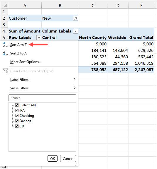
Click the ‘Sort and Filter’ button (down arrow icon) in cell A5, next to the ‘Row Labels’ header.

The above step opens a drop-down menu.

Select the Sort A to Z option on the drop-down menu.

Note: Choose the ‘Sort Z to A’ option to sort the rows in descending alphabetical order by row labels.

The above step sorts the rows in the Pivot Table in ascending alphabetical order based on the row labels.

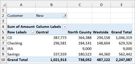
Notice that in cell A5 the ‘Sort and Filter’ button’s icon changes to indicate that the row labels are sorted in ascending alphabetical order.

Method #4: Use a Custom List to Reorder Rows in a Pivot Table

You can reorder rows in a Pivot Table using a custom list to sort the row labels in a custom order.

You want the row labels to appear in the following order: Savings, Checking, CD, and IRA.

Here’s how to do it:

Step #1: Create the Custom List

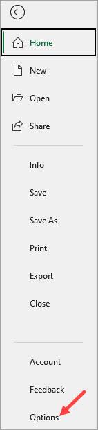
Click the File button on the Ribbon to open the Backstage view.
Click Options on the left panel of the Backstage view.

The above step opens the Excel Options dialog box.

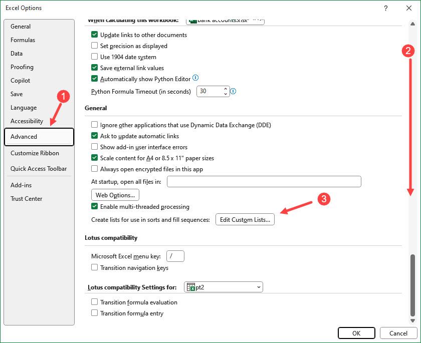
On the Excel Options dialog box, click Advanced on the left panel, scroll down to the General section, and click the Edit Custom Lists button.

The above step opens the Custom Lists dialog box.

On the Custom Lists dialog box, ensure ‘NEW LIST’ is selected on the ‘Custom lists’ list box, type your custom list on the ‘List entries’ list box, click the Add button, and click OK.

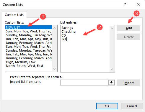
The above step adds your custom list at the bottom of the pre-existing custom lists on the ‘Custom lists’ list box.

Click OK on the Excel Options dialog box.

Step #2: Use the Custom List to Reorder Rows in the Pivot Table

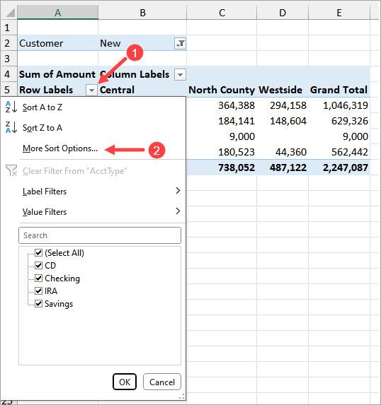
Click the Sort and Filter button in cell A5 of the Pivot Table and select ‘More Sort Options’ on the drop-down menu.

The above step opens the Sort dialog box.

On the Sort dialog box, select the ‘Ascending (A to Z) by:’ option and click the ‘More Options’ button.

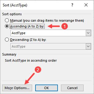
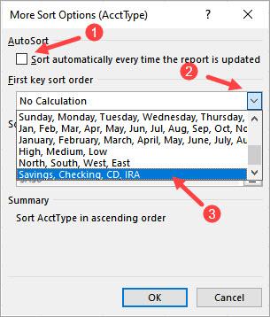
select the 'Ascending (A to Z) by:' option

The above step opens the ‘More Sort Options’ dialog box.

On the ‘More Sort Options’ dialog box, uncheck the ‘Sort automatically every time the report is updated’ checkbox, open the ‘First key sort order’ drop-down list, select the custom list you created in step 4 above, and click OK.

uncheck the 'Sort automatically every time the report is updated' checkbox

Click OK on the Sort dialog box.

Excel rearranges the row labels and the rows in the Pivot Table according to the order in the custom list.

I have shown you how to reorder rows in a Pivot Table using drag and drop, Move options, and sorting with Excel built-in options and a custom list. I hope you found the tutorial helpful.

Other Excel articles you may also like: