Opposite of Concatenate in Excel (Reverse Concatenate)

To concatenate in Excel is to combine data from multiple cells into one cell.

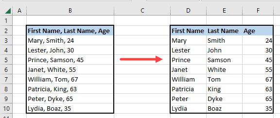
Therefore, to do the opposite of concatenation or reverse concatenation is to split the contents of individual cells into separate cells, as shown in the example below:

Opposite of Concatenate in Excel (Reverse Concatenate)

This tutorial shows five techniques for doing the opposite of concatenation or reverse concatenation in Excel.

Table of Contents

Why Do Reverse Concatenation?

Before we delve into the techniques for reverse concatenation, we must first understand the operation’s benefits.

There are several reasons why we might need to reverse concatenate our dataset. The reasons include the following:

More straightforward data analysis – When we split the data in individual cells into separate cells, it becomes easier to do data analysis and perform data manipulation operations such as filtering, sorting, and creating PivotTables.
Better organization – Data split into separate cells is more readable and organized.
Improved accuracy – Data split into separate cells helps improve data accuracy by minimizing the chances of errors in data entry and data manipulation.

Let’s dive into the tutorial and learn the techniques for reverse concatenation.

Method #1: Use Flash Fill to Do the Opposite of Concatenate in Excel

Flash Fill is a feature in Excel that allows us to fill in data based on the patterns we specify automatically.

Consequently, we can use this feature to do the opposite of concatenating in Excel.

Let’s consider the following dataset showing the first names, last names, and ages of particular faculty of a specific university.

We want to use Flash Fill to split the data in column A into columns B, C, and D.

We use the steps below:

Select cell B2 and type in the first name of the first staff, “Mary.”
Select cell B3 and type in the first name of the second staff, “Lester.”

Notice that as we begin to type the first name of the second staff, Flash Fill detects what we want to do and gives us suggestions for the following entries in grey:

If the suggestions are correct, we press Enter to accept them, and the entries are entered automatically into the cells.

Note: If Flash Fill does not give us suggestions for the following entries or gives incorrect suggestions, we must finish typing in the first name of the second staff, “Lester,” and then continue with the next steps:

Select cell B4.

On the Data tab, in the Data Tools group, click the Flash Fill button.

All the first names of the faculty are filled in automatically.

Note: Instead of using the Flash Fill button on the Data tab, we can press the shortcut Ctrl + E and achieve the same results.

We repeat steps 1 to 5 to fill in the last names and then the ages of the staff.

Note: Flash Fill is not dynamic, therefore, if there is a change in the source data in column A, we will have to redo Flash Fill in columns B, C, and D to update the data.

We no longer need the source data in column A; therefore, we delete the column by clicking the letter column header to select the entire column, right-clicking the selection, and choosing Delete on the shortcut menu that appears.

We end up with a dataset where the data in one column is split into three separate columns.

Method #2: Use the Text to Columns Feature to Do Reverse Concatenation in Excel

The Text to Columns feature in Excel is used to split a single column of data into several columns based on a specified delimiter, such as a tab, comma, or space.

Therefore we can use this feature to do the opposite of concatenate or reverse concatenate data in Excel.

Presume we have the following dataset showing the first names, last names, and ages of particular faculty of a specific university.

We want to use the Text to Columns feature to split the data into three columns.

We apply the following steps:

Select the cell range A1:A9 containing the dataset.

On the Data tab, in the Data Tools group, click the Text to Columns button.

On the Convert Text to Columns Wizard – Step 1 to 3 dialog box, select Delimited and click Next.

Notice the preview of the selected data at the bottom of the dialog box.

On the Convert Text to Columns Wizard – Step 2 to 3 dialog box, uncheck the Tab delimiter, select the Comma delimiter separating the data we want to split, and click Next.

Notice the data preview at the bottom of the dialog box.

On the Convert Text to Columns Wizard – Step 2 to 3 dialog box, leave the default options as is, and click Finish.

The reverse of concatenation takes place, and the data is split into three columns:

Method #3: Use the TEXTSPLIT Function to Do the Opposite of Concatenate in Excel

The TEXTSPLIT function splits text strings using row and column delimiters.

It works the same way as the Text to Columns feature in Method #2 but in a formula form.

Therefore we can utilize it to do reverse concatenation in Excel. However, it is only available in Excel 365.

The Syntax and Arguments of the TEXTSPLIT Function

Before we can apply the TEXTSPLIT function in doing the opposite of concatenation in Excel, we must understand its syntax and the arguments it takes.

The syntax of the TEXTSPLIT function is as follows:

TEXTSPLIT(text,col_delimiter,[row_delimiter],[ignore_empty], [match_mode], [pad_with])

The function takes two required arguments and four optional ones, as enumerated below:

text This is mandatory and is the text we want to split.
col_delimiter This is required and is the text marking the point where to spill the text strings across columns.
row_delimiter This is optional and is the text marking the point where to spill the text strings down rows.
ignore_empty This is optional and defaults to FALSE, creating an empty cell in place of a consecutive delimiter. We specify TRUE when we want to ignore successive delimiters.
match_mode This is optional and defaults to 0 (zero), doing a case-sensitive match. We specify 1 to perform a case-insensitive match.
pad_with This is optional and is the value to pad the result. It defaults to #N/A.

Let’s now apply the function to split the data in column A of our example dataset below into three columns.

We use the below steps:

Select cell C1 and type in the formula below:

=TEXTSPLIT(A1,",")

Click Enter to get the result of the formula.
Drag the fill handle to copy the formula down the column.

The data in column A is split into columns C, D, and E.

TEXTSPLIT doing opposite of concatenation

Note: The TEXTSPLIT function is dynamic, so if there are changes in the source data in column A, they are reflected automatically in columns C, D, and E.

Deleting the Source Data

If we want to delete column A, which contains the source data, we must first convert the data in columns C, D, and E into values; otherwise, we get the #REF! error as shown below:

Deleting source data would give ref error

To convert the data in columns C, D, and E into values, we use the steps below:

Select the cell range C1:E9.

Press Ctrl + C to copy the data.

Notice the “marching ants” border around the selection, indicating that the data is copied to the clipboard.

Press Ctrl + Alt + V to activate the Paste Special dialog box.
On the Paste Special dialog box, select Values and click OK.

The formulas in the cell range C1:E9 have been converted into values.

Notice the green Error Indicators in cell range A2:A8. They appear because the numbers in the cells are stored as text strings. Do the following steps to convert the text strings into numbers:

Select the cell range E2:E9 and notice the Smart Tag indicator (yellow triangle) next to cell E2.

The error description pops up when we hover the cursor over the Smart Tag.

Error description number formatted as text

Click the down arrow on the Smart tag and choose Convert to Number on the drop-down.

The text strings in the cell range E2:E9 are converted immediately to numbers.

Now, we can safely delete columns A and B from the dataset by clicking the letter header of column A, dragging across to the letter header of column B, right-clicking the selection, and choosing Delete on the shortcut menu that appears.

The resultant dataset with data split into columns A, B, and C appears in the cell range A1:C9.

Resulting dataset after reverse concatenate

Method #4: Using Combination of TRIM, MID, SUBSTITUTE, REPT, and COLUMN Functions To Do the Opposite of Concatenate in Excel

We can use a formula that combines the TRIM, MID, SUBSTITUTE, REPT, and COLUMN functions to split the contents of individual cells into separate cells.

The following is a brief description of the text functions:

TRIM Removes all the spaces from a text string except for the single spaces between words.
MID Returns the text from the middle of a text string given the starting position and length.
SUBSTITUTE Replaces the existing text string with new text in a text string.
REPT Repeats text a given number of times.
COLUMNS Indicates the number of columns in a cell reference or array.

Let’s now show how to use a formula combining the text functions to split the contents of column A in the following dataset into separate columns.

We use the following steps:

Select cell C1 and type in the below formula:

=TRIM(MID(SUBSTITUTE($A1,",",REPT(" ",999)),COLUMNS($A:A)*999-998,999))

Click Enter on the Formula bar.

Drag the fill handle across to cell E1.

Drag the fill handle down to cell E9.

Convert the contents of the cell range C1:E9 to values as explained in Method #3.
Convert the text strings in the cell range E2:E9 to numbers, as illustrated in Method #3.
Delete columns A and B as explained in Method #3.

The contents of the original dataset have been split into columns A, B, and C.

Explanation of the Formula

=TRIM(MID(SUBSTITUTE($A1,",",REPT(" ",999)),COLUMNS($A:A)*999-998,999))

REPT(” “,999) The REPT function repeats the space character 999 times inside the SUBSTITUTE function.
SUBSTITUTE($A1,”,”,REPT(” “,999)) The SUBSTITUTE function substitutes comma for the 999 spaces generated by the REPT function.
MID(SUBSTITUTE($A1,”,”,REPT(” “,999)),COLUMNS($A:A)*999-998,999) The MID function returns the title, “First Name,” plus several space characters, totaling 999 characters.
TRIM(MID(SUBSTITUTE($A1,”,”,REPT(” “,999)),COLUMNS($A:A)*999-998,999)) Finally, the TRIM function removes all the unnecessary spaces after the title “First Name.”

Method #5: Use a Combination of LEFT, MID, FIND, and LEN Functions to Do the Opposite of Concatenate in Excel

We can apply formulas combining the LEFT, MID, FIND, and LEN text functions to reverse concatenate in Excel.

The following is a short description of the text functions:

LEFT Returns the specified number of characters from the start of a text string.
MID Returns the text from the middle of a text string given the starting position and length.
FIND Returns the starting position of one text string within another. The function is case-sensitive.
LEN Returns the number of characters in a text string.

We use the following dataset to show the application of formulas combining the mentioned text functions in performing the opposite of concatenation in Excel.

We use the below steps:

Select cell C2 and type in the formula below:

=LEFT(A2,FIND(",",A2)-1)

Click Enter on the Formula bar.

Drag or double-click the fill handle to copy the formula down the column.

Select cell D2 and type in the below formula:

=MID(A2,FIND(",",A2)+1,LEN(A2))

Click Enter on the Formula bar.

Double-click or drag the fill handle to copy the formula down the column.

The contents of column A have been split into columns C and D.

Explanation of the formulas

=LEFT(A2,FIND(“,”,A2)-1)

FIND(“,”,A2)-1 The FIND function returns the starting position of the comma in the target text string. The number is reduced by 1, resulting in the number of characters of the first name preceding the comma.
LEFT(A2,FIND(“,”,A2)-1) The LEFT function uses the value from the previous step to extract the first name from the target text string.

=MID(A2,FIND(“,”,A2)+1,LEN(A2))

FIND(“,”,A2)+1 The FIND function returns the starting position of the comma in the target text string. The number is increased by 1, resulting in the starting position of the last name.
LEN(A2) The LEN function returns the number of characters in the target text string.
MID(A2,FIND(“,”,A2)+1,LEN(A2)) The MID function uses the values returned in the previous two steps to extract the last name, which starts after the space character following the comma.

This tutorial showed five methods for doing the opposite of concatenate or reverse concatenate in Excel. We hope you found the tutorial helpful.

Other Excel articles you may also like: