As we work with Excel, we may sometimes need to combine two columns and separate them with characters such as a space or a comma.
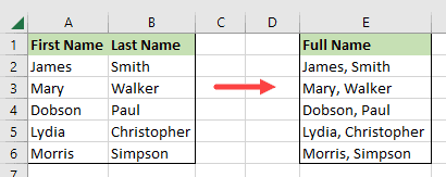
Below is an example where I got the data where I had the first and the last name in separate columns, and I wanted to combine the two columns while adding the comma in between the names.
In this tutorial, I have covered six simple methods you can use to combine two columns in Excel while separating them with a comma (or space or any other delimiter).
Let’s dive in!
Method #1: Combine Two Columns in Excel Using the Ampersand (&) Operator
The ampersand (&) operator is used in Excel to join or concatenate values.
When we use the ampersand operator to join values the result is always text strings, even when the values are numbers.
Suppose we have the following dataset displaying the first name and the last name in columns A and B, respectively.

We want to combine the values in the two columns into column C using the ampersand operator.
Below are the steps to do this:
- Select cell C2 and type in the following formula:
=A2&", "&B2
Notice that the comma is in double quotes, followed by a single-space character. We are doing this as we want the names to be separated by a comma followed by a space character

- Click the Enter button on the formula bar to enter the formula (or press the Enter key).

- Copy the formula down the column by double-clicking on the fill handle or holding and dragging it down.
Below is the result where the values in column A and column B are combined, and we get the result in column C.

Since we have used a formula, in case you make any changes to the names in column A or column B, it will automatically be reflected in column C.
In case you do not want to keep the first and the last names and only want to keep the resulting full name, you first need to remove the formula and only keep the values (so that your resulting values remain as is when you delete columns A and B).
I have a detailed tutorial on how to delete the formulas and keep the values.
Also read: Append Text To End Of Cell in Excel
Method #2: Combine Two Columns in Excel Using the CONCAT Function
We can use Excel’s built-in CONCAT function to concatenate or combine a range or a list of text strings.
Assume we have the following dataset displaying the first name in column A and the last name in column B.

We want to combine the values in the two columns in column C using the CONCAT function.
You can follow the steps below to do this:
- Select cell C2 and type in the formula below:
=CONCAT(A2,", ",B2)

- Enter the formula by clicking the Enter button on the formula.

- Drag down or double-click the fill handle to copy the formula down the column.

The CONCAT function is just like using the & operator (covered before this method), where it combines all the arguments that are supplied to it.
In the above formula, we wanted to combine columns A and B while separating the text values in the columns with a comma and a space. So we entered the references of the columns as the first and the third argument while adding the delimiter as the second argument.
Remember that the comma followed by the space character needs to be in double quotes, as we want Excel to use it as is as text.
Also read: How to Swap Columns in Excel?
Method #3: Combine Two Columns With Line Breaks Using the CONCAT and CHAR Functions
If we want to combine two columns with line breaks, we can vary the previous method by including the CHAR function.
The CHAR function returns the character specified by the code number from the character set of the device we are using. In this case, we shall use the code number 10 to return the line break character.
Suppose we have the following dataset that has the first name in column A and the last name in column B.

We want to combine the two columns into column C with a line break.
We proceed as follows:
- Select cell C2 and type the following formula:
=CONCAT(A2,",",CHAR(10),B2)
Notice that there is no space after the comma in double quotes.

- Click the Enter button on the formula bar to enter the formula.

- Double-click or drag down the fill handle to copy the formula down the column.

While the above steps did combine the names in columns A and B, it’s still not in the desired format. We wanted the names to be on separate lines in the same cell.
While we have already added the line break character by using the CHAR(10) as the delimiter, for the names to actually appear on separate lines, you need to apply the wrap text formatting to the cells
To do that, select names in column C and then click on the Wrap Text icon in the ribbon (it’s in the Home tab in the alignment group)

As soon as you apply the wrap text formatting, you will notice that the names now appear on separate lines in the same cell.

Also read: How to Press Enter in Excel and Stay in the Same Cell?
Method #4: Combine Two Columns in Excel Using the TEXTJOIN Function
We can use Excel’s built-in TEXTJOIN function to concatenate or combine a range or a list of text strings using a delimiter or separator.
TEXTJOIN is a new function added in Excel 2019, so if you cannot find it in your Excel version, you will not be able to use this method
Imagine we have the following dataset displaying the first and last names in columns A and B, respectively.

We want to combine the text values in columns A and B and get the result in column C using the TEXTJOIN function.
We can do that using the following steps:
- Select cell C2 and type in the following formula:
=TEXTJOIN(", ",TRUE,A2,B2)

- Enter the formula by clicking the Enter button on the formula bar.

- Drag down or double-click the fill handle to copy the formula down the column.

Explanation of the formula
The TEXTJOIN function has the following syntax:
TEXTJOIN(delimiter, ignore_empty, text1, [text2]…)
In the formula, we first specified “, “ as the delimiter (which would be added between the values of the combined columns).
The second argument is set to TRUE, which tells the formula that in case of encounters any blank cells, these should be ignored.
After the delimiter and the ignore_emptry arguments, the two arguments are the cell references of the cells that we want to combine (A2 and B2 in this example)
Also read: Generate All Possible Combinations from Two Lists
Method #5: Combine Two Columns in Excel Using the Flash Fill Feature
The Flash Fill is a really helpful feature that works by recognizing the pattern based on one or two inputs from the user.
Once it recognizes the patterns, it can fill the entire column following the same pattern.
We can use the Flash Fill feature to combine two columns in Excel.
Assume we have the following dataset displaying the first name in column A and the last name in column B.

We want to combine the values in the two columns into column C using Flash Fill.
Below are the steps to do this:
- Select cell C2 and type in the value James, Smith, and press Enter.
- In cell C3, type in the value Mary, Waker.
Notice that as you enter the value in cell C3 Flash Fill detects a pattern in the data and gives you suggestions for the next data in grey.

If the suggestions are correct, press Enter to accept them.

Note: If Flash Fill does not give you the suggestions in grey, finish typing the value in cell C3 then do the following:
- Select the range C2:C6 as follows:

- On the Data tab, in the Data Tools group, click the Flash Fill button:

Alternatively, you use the keyboard shortcut Ctrl + E.
The two columns are combined in column C.

Method #6: Combine Two Columns in Excel Using a User Defined Function
Another way we can combine two columns in Excel is by using a User Defined Function created in Excel VBA.
Suppose we have the following dataset displaying the first and last names in columns A and B, respectively.

We want to combine the values in column A and column B in column C using a User Defined Function.
We apply the following steps:
- Open the worksheet containing the dataset.
- On the Developer tab, in the Code group, click Visual Basic to open the Visual Basic Editor.

Alternatively, you can open the Visual Basic Editor by pressing Alt + F11.
- On the Insert menu, select Module to insert a module.

- Enter the following function code in the module code window:
'Code developed by Steve Scott from https://spreadsheetplanet.com
Function COMBINECOLUMNS(Col1 As Range, Col2 As Range, Optional Sign As String = ", ") As String
Dim Rng As Range
Dim resultString As String
If Col1 <> "" Then
    If Col2 <> "" Then
        resultString = Col1 & Sign & Col2
    Else
        resultString = Col1
    End If
ElseIf Col2 <> "" Then
        resultString = Col2
    Else
        resultString = ""
    End If
COMBINECOLUMNS = resultString
End Function- Click the View Microsoft Excel icon on the toolbar to switch to the active worksheet containing the dataset.

Alternatively, you can switch to the active worksheet by pressing Alt + F11.
- Select cell C2 and type in the formula below:
=COMBINECOLUMNS(A2,B2)

Notice that Excel IntelliSense detects the User-Defined Function (and it will show up as soon as you type the first few alphabets of the function name:

- Click the Enter button on the formula bar to enter the formula.

- Drag down or double-click the fill handle to copy the formula down the column.

I’ve created the above VBA code to combine two columns and have specified the delimiter as “, “.
In case you want to combine more than two columns, you can easily modify this code to suit your needs.
In this tutorial, I’ve covered six methods you can use to combine columns in Excel. The easiest way to do this would be by using simple formulas such as one using & operator or the CONCAT or TEXTJOIN functions.
I have also covered how you can do this using the new Flash Fill feature or a simple VBA code to combine multiple columns.
Other Excel articles you may also like:
- How To Combine Date and Time in Excel
- Switch First and Last Name with Comma in Excel (Reverse Names)
- How to Apply Formula to Entire Column in Excel?
- How to Flip Data in Excel (Columns, Rows, Tables)?
- How to Merge Two Excel Files?
- How to Merge First and Last Name in Excel
- Remove Middle Name from Full Name in Excel
- How to Remove Commas in Excel (from Numbers or Text String)
- How to Separate Names in Excel
- Opposite of Concatenate in Excel (Reverse Concatenate)