When working with formulas, there is always a possibility that someone (or even you) may delete a cell (or clear the contents of a cell/range) that has formulas in it.
Wouldn’t it be better if these cells with formulas are highlighted or formatted in a way that makes these stand out? This would help ensure you don’t end up deleting these cells by mistake.
In this tutorial, I will show you how to auto-format formulas in Excel (i.e., highlight the cells with formulas).
So let’s get started!
Autoformat Formulas using Conditional Formatting
The easiest way to autoformat cells with formulas is to use conditional formatting.
If you can somehow identify cells that have formulas, you can easily format these differently using conditional formatting.
And this is where you can use the ISFORMULA function, a function that was introduced in Excel 2013.
The ISFORMULA function checks whether a cell has a formula in it or not, and if it has a formula, then it returns TRUE (else FALSE).
Below are the steps to use this function in Conditional Formatting to autoformat formulas in Excel:
- Select the dataset in which you want to format the cells with formulas
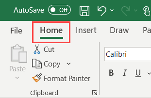
- Click the Home tab
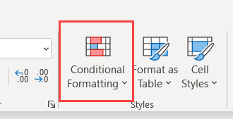
- In the Styles group, click on Conditional Formatting
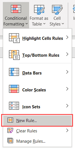
- Click on New Rule
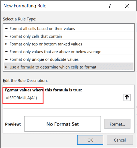
- In the New Formatting Rule dialog box that opens, select ‘Use a formula to determine which cells to format’
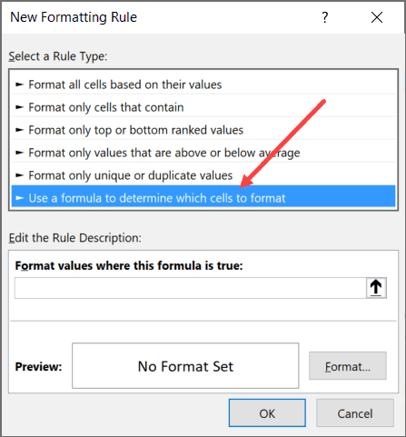
- In the formula field, enter the formula =ISFORMULA(A1)
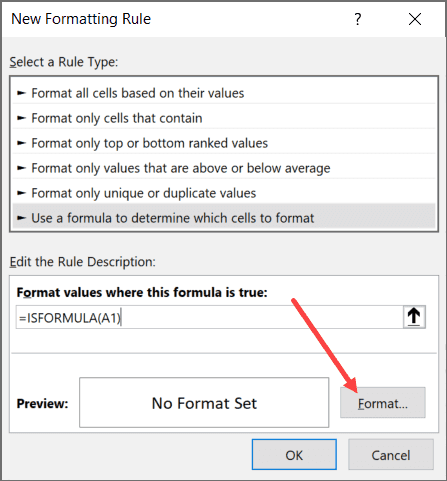
- Click on the Format button
- In the Format Cells dialog box that opens, specify the formatting that you want to apply to the cells with formulas. In my case, I am using the orange cell fill color
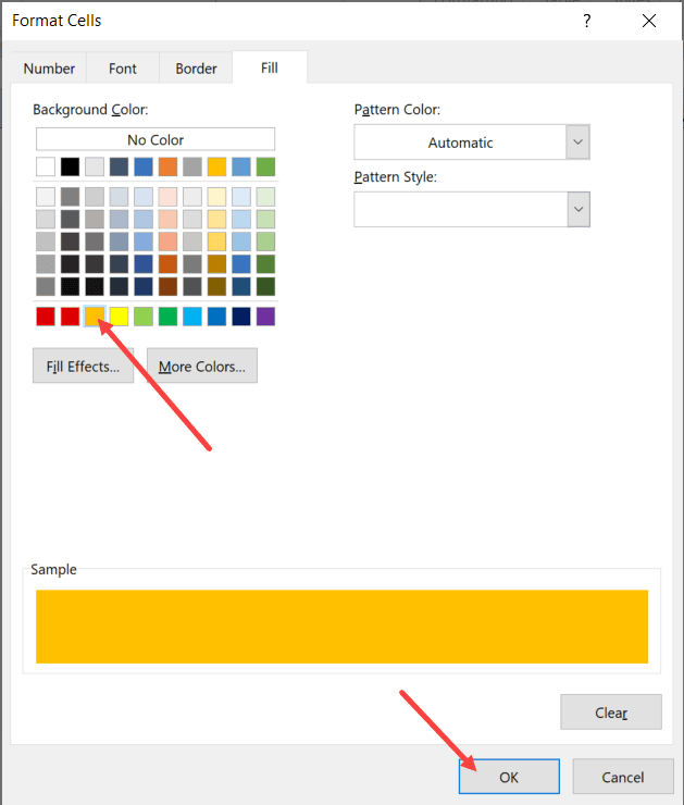
- Click OK
The above steps would instantly autoformat all the cells that have a formula in it.
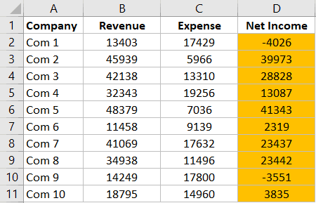
Not only this, in case you change any of the cells and add a formula to it, the color would automatically change. Since conditional formatting is dynamic and checks for each cell every time there is a change in the worksheet, the above steps make sure cells are automatically highlighted.
While this is my preferred method to autoformat formulas in Excel, there is another way as well.
Also read: How to Strikethrough in Excel (5 Ways + Shortcuts)
Autoformat Formulas using Go To Special
Unlike the Conditional formatting method, this one is not dynamic.
So when you do this once, it will select all the cells with formulas and you can format them at one go. But if now you change any cell and add a formula, that cell will not get highlighted.
Below are the steps to use Go To Special to select all cells with Formulas and then format these:
- Select the dataset in which you want to format the cells with formulas
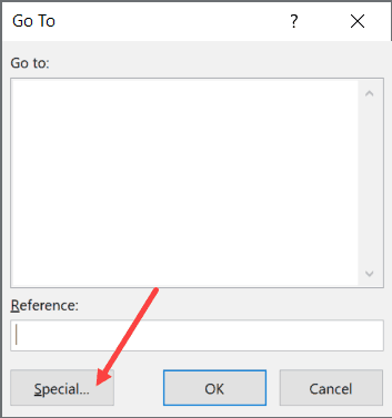
- Hit the F5 key – this will open the Go To dialog box
- Click on the Special button
- In the Go To Special dialog box, Click on Formulas
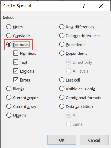
- Click OK
The above steps would select all the cells that have formulas in them.
Once these cells are selected, you can apply whatever formatting you want. For example, you can apply a cell color or can change the font to bold.
As I mentioned, now, if you add a new formula to the range, it will not get autoformatted. You will have to repeat the same process again.
Also read: How to Remove Formulas in Excel (and keep the data)
Format Formulas using VBA
Another quick method to quickly format cells with formulas is by using VBA.
This method does exactly the same thing as the previous method (using Go To Special), but with a single line of code.
Below is the VBA code that will instantly highlight all the cells that have formulas in it in yellow color:
Selection.SpecialCells(xlCellTypeFormulas, 23).Interior.Color = vbYellow
This code first selects all the cells that have formulas and then applies the yellow color (specified by vbYellow).
Here are the steps to use this VBA macro code:
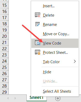
- Right-click on the active sheet tab name (the one where you have the data with formulas that you want to format).
- Click on View Code
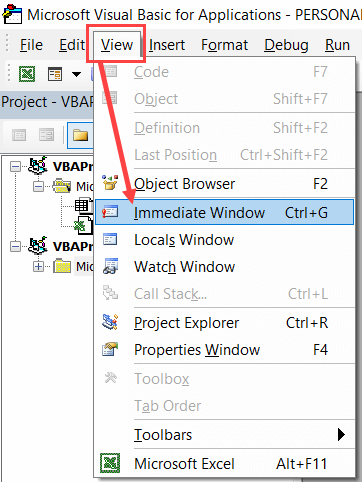
- If you don’t see the ‘Immediate window’ in the VB Editor already, click on the ‘View’ option in the menu and then click on ‘Immediate Window’
- Copy and paste the above VBA code in the ‘Immediate Window’
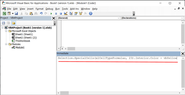
- Place the cursor at the end of the line
- Hit the Enter key
The above code first identifies all the cells with formulas and then applies the yellow color. You can modify the code in case you want to apply some other type of formatting.
So these are two simple ways to quickly autoformat formulas in Excel.
Hope you found this tutorial useful!
You may also like the following Excel tutorials:
- How to Format Phone Numbers in Excel
- How to Clear Contents in Excel without Deleting Formulas
- How to Delete a Comment in Excel (or Delete ALL Comments)
- Excel Showing Formula Instead of Result
- SUMPRODUCT vs SUMIFS Function in Excel
- How to Convert Decimal to Fraction in Excel
- How to Shade Every Other Row in Excel
- How to Autofill Dates in Excel (Autofill Months/Years)
- How to Apply Comma Style in Excel
- How to Increase/Decrease Indent in Excel? (Easy Shortcut)