If you need to subtract a single value from a range of cells at the same time, there are multiple ways can do this in Excel.
For example, suppose you have the scores of students and you want to deduct 5 marks from all scores, you can do that using a simple formula (and some other simple methods that we will see this tutorial)
When you need to subtract multiple cell values from a particular number, the best way to do it is to put the number in one of the cells (on the same sheet or a different sheet) and apply a simple formula.
In this Excel tutorial, I will show you three useful tricks that you can use to subtract multiple cells from one cell in Excel.
Among these, you will see how to tweak your formula to work with this problem, a cool trick using the Paste Special feature and if you’re up to it, some VBA coding!
So let’s get started!
Subtract Multiple Cells from a Cell using a Formula
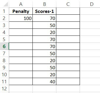
Let us say you have a dataset as given below (cells B2:B11) and you want to subtract each of these values from the value in cell A2.
The easiest way to do this is by using a simple subtraction formula.
Here are the steps to do this:
- Click on a cell of an empty column, say C2 and type the following formula in the formula bar: =A2-B2
- Lock the cell location A2 by clicking either before, after, or in between the reference to A2 and pressing the F4 Key. Notice that the cell location A2 changes to $A$2. You can also manually add these dollar signs if you want.
- Press the Return/Enter key on your keyboard
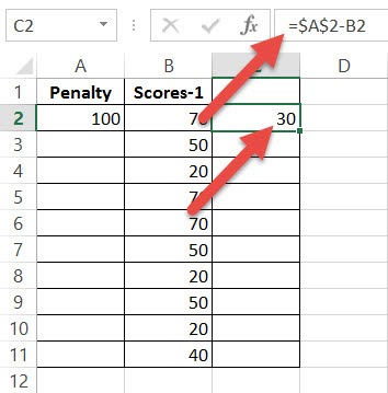
- Drag down the fill handle on the lower-right corner of cell C2 to copy the formula for all cells (C2:C11). You will now get a whole column of cells containing the difference between cell A2 and cells B2:B11.
Note: Using the formula method has an advantage – which is that the result is dynamic. In case you change the value in cell A2, the resulting data would automatically update. And one disadvantage if this method is that it would need an additional column for you to get the result (which is not such a big problem in most cases).
In case you don’t want the result to be linked to A2 cell, you can convert these formulae into values.
Now, if you are wondering why we pressed F4 and changed the reference of A2 to $A$2.
The reason for this is that we wanted to make the reference to cell A2 an absolute reference rather than a relative reference.
So to make this even clearer, let me quickly tell you about absolute and relative references.
Difference between Absolute and Relative Cell References in Excel
Absolute and relative cell references react differently when copied to other cells. They are also represented differently in formulas. For example, a relative reference to a cell in column A, row 1 is represented as A1. An absolute reference to the same cell, however, is represented as $A$1.
By default, all cell references are relative references. To convert a cell reference to an absolute reference, you need to add a dollar ($) sign to it or simply press the F4 key when the cursor is on, before or after the reference.
When you copy and paste a cell with a relative reference, the cell reference is adjusted according to the location it is pasted in. However, a relative reference never changes and always refers to the same cell location, irrespective of where it is pasted.
For example, if you copy the formula =A1 – B1 from row 1 to row 2, the formula will become =A2 – B2. However, if you copy the formula =$A$1 – B1 from row 1 to row 2, the formula becomes $A$1 – B2.
Notice, the reference in the first operand did not change, since it was specified as an absolute reference ($A$1). The reference to the cell in the second operand, however, changed from B1 to B2.
In our example, we want the reference to cell A2 to remain constant when the formula is copied and filled to other cells in column C. Therefore, we converted the reference A2 to an absolute reference.
Also read: Get Percentage Difference Between Two Numbers in Excel
Subtract Multiple Cells from a Cell using Paste Special
As I said, there are multiple ways to skin this cat in Excel.
So here is another simple method to subtract a range of cells from a specific value.
If you want to subtract, say cells B2:B11 from the cell A2, and replace the difference back in cells B2:B11, here’s another cool trick that you can use:
- Select cell A2.
- Press CTRL+C to copy (or right-click and then select copy)
- Select cells B2:B11
- Right-click anywhere on your selection and click on the Paste Special option. This will open the Paste Special dialog box.
- In the Paste Special dialog box, select Subtract (under the Operation options).
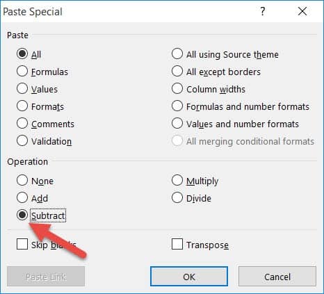
- Click OK.
That’s it!
You would notice that the numbers in the selected range (B2:B11) has changed where the resulting data is now after the value in cell A2 has been subtracted.
You can now delete the value in cell A2 if you want (as the result is not linked to this cell).
In case you want to hold on to the original data, make a copy of the cells, and then perform the above operation on the copied cells.
Subtract Multiple Cells from a Cell using VBScript
If you are up for a little coding and are comfortable with using VBscript, here’s a third method that you can apply.
Before you start, here’s the VBA code that we are going to be using:
Sub SubtractfromCell()
For Each cell In Selection
cell.Value = Range("E2") - cell.Value
Next cell
End SubKeep the CTRL key on your keyboard pressed and select all the cells B2:B11.Copy this code and keep it somewhere safe, like in a notepad file so that you can reuse it later.
- From the Developer Menu Ribbon, select Visual Basic.
- Once your VBA window opens, Click Insert->Module. Copy the code given above and paste it into the Module Window.
- Run the code by clicking on the button from the toolbar on top.

- Close the VBA window.
When you return to your worksheet, you will find all your selected cell values replaced with their individual differences from cell A2.
Beware though, this method permanently changes the values in your selected cells. So, in case you want to hold on to the original data, make a copy of your data in a separate column, and then perform the operation.
In the above method, we created a macro that goes through each selected cell and subtracts the value from the value in cell A2.
If you want to subtract these cells from some other cell, simply replace “A2” in line 3 to the reference to your required cell.
This method has merit when you have to subtract multiple such columns (or range of cells) the value in a specific cell. Instead of doing the formula or using paste special multiple times, you can do it faster with VBA.
Conclusion
In this Excel tutorial, we looked at three different ways in which you can subtract multiple cell values from one cell in Excel. Among these, we saw how you could use a formula, the Paste Special feature, and a VBScript.
You can use whichever of the above techniques you feel comfortable with. If you know of any other more effective techniques, do let us know in the comments.
Other Excel tutorials you may find useful:
Very helpful information. Thanks