Reversing a string may not have many real-world applications, especially when working with spreadsheets. That is why you will not find any built-in function for this in Excel.
But there might be cases where you need to reverse a string, for whatever reason. Maybe you need to generate a special code, maybe you need to see if a string is a palindrome, or maybe you just want to do it for fun.
Even though there aren’t any built-in Excel functions for string reversal, there are a number of different ways to do this. You can use either a formula or a script written in VBA.
In this tutorial, we will see two ways to reverse a text string using a formula. If you like to use macros, then we also have a VBA script to help you reverse multiple strings quickly.
Reversing Text String using Text Formulas
Let us first understand the main process involved in reversing a string.
Let’s say you have a single cell with text that you want to reverse.
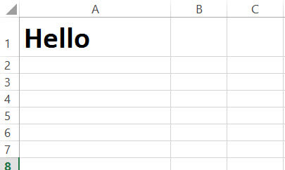
To reverse the string “Hello” in cell A1, follow these steps:
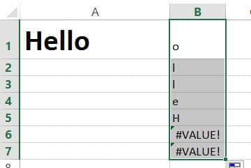
- In cell B1, type the following formula: =MID($A$1,LEN($A$1)-ROW(B1)+1,1). This should return the last character in the given string, which is “o”.
- Drag the fill handle down (situated at the bottom right of cell B1) until you start seeing “#VALUE!”.

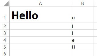
- You should now see each character of the string in “Hello” in each cell of column B, but reversed. Clear any cells containing “#VALUE!”. Here’s what you should finally see in our example:

- After the last cell of column B, i.e. in cell B6, type the formula: =TRANSPOSE(
- Drag and select the cells B1 to B5.
- Close the parentheses for the TRANSPOSE formula.
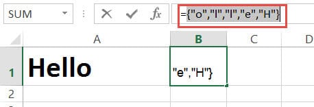
- Now select the whole formula in the formula bar and press F9 on your keyboard. This should display the values of each cell from B1 to B5, separated by commas and the whole thing should be surrounded by curly brackets: {“o”,”l”,”l”,”e”,”H”}.
- Remove the opening and closing curly brackets.
- Type “CONCATENATE”, followed by opening parentheses after the equal to sign.
- Close the parentheses after “H”.
- Press the return key.
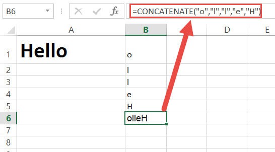
You should now see the reverse of the string “Hello” in cell B6.
What happened here?
Now let us look at what the formula did.
=MID($A$1,LEN($A$1)-ROW(B1)+1,1)
The function LEN($A$1) returns the length of the string in cell A1. We don’t want this cell reference to change when copied to the cells below B1, so we locked the cell reference by adding ‘$’ signs to it. The length of the string “Hello” is 5, so this function will return the value, ‘5’.
The function ROW(B1) simply returns the row number of cell B1. We might as well have typed ‘1’ instead of ‘ROW(B1)’, but wanted this value to change each time it was copied to a new cell. So when it’s copied to cell B2, it changes to value ‘2’. When copied to cell B3, it changed to value ‘3’ and so on.
Now, LEN($A$1)-ROW(B1)+1 gives us the value ‘5’, which is the index of the last character in “Hello”.
The function MID() returns the characters at a given index. It takes three parameters – A string or reference to a string, an index, and the number of characters to return starting at that index.
Here, the formula =MID($A$1,LEN($A$1)-ROW(B1)+1,1) takes the reference to cell A1 as the first parameter, the index, 5 as the second parameter and the number 1, as the third parameter. So the formula returns the character at index 5 of cell A1. This means we get the value “o” – the last character of the string.
Here’s what’s happening when you break down the formula:
- =MID($A$1,LEN($A$1)-ROW(B1)+1,1)
- =MID($A$1, 5 – 1 + 1, 1)
- =MID($A$1, 5, 1)
- =”o”
What happens when the formula is copied to cell B2?
In cell B2, the formula now changes to:
=MID($A$1,LEN($A$1)-ROW(B2)+1,1)
Here’s what’s happening when you break down the formula:
- =MID($A$1,LEN($A$1)-ROW(B2)+1,1)
- =MID($A$1, 5 – 2 + 1, 1)
- =MID($A$1, 4, 1)
- =”l”
What happens when the formula is copied to cell B5?
In cell B5, the formula now changes to:
=MID($A$1,LEN($A$1)-ROW(B5)+1,1)
Here’s what’s happening when you break down the formula:
- =MID($A$1,LEN($A$1)-ROW(B5)+1,1)
- =MID($A$1, 5 – 5 + 1, 1)
- =MID($A$1, 1, 1)
- =”H”
So the function returns the first character of the string in A1.
Also read: 100 Useful Excel VBA Macro Codes Examples
Reverse a Text String in Excel using TRANSPOSE Formula
Although the above method works fine, it is not very practical as you would need to involve a whole lot of cells in your sheet. We demonstrated the above method just to break down the technique and make it easy for you to understand what’s happening.
Here’s a shortened down and more practical version of the above technique:
- In cell B1, type the formula:
=TRANSPOSE(MID(A1,LEN(A1)-ROW(INDIRECT("1:"&LEN(A1)))+1,1)) in cell B1. - Select the entire formula in the formula bar and press F9 on your keyboard.
- This should display each character of your string, reversed and separated by commas. The whole thing should be also surrounded by curly brackets, which means this is an array: {“o”,”l”,”l”,”e”,”H”}.

- Remove the opening and closing curly brackets.
- Type “CONCATENATE”, followed by opening parentheses after the equal to sign.
- Close the parentheses after “H”.
- Press the return key.

You should now see the reverse of the string “Hello” in cell B1. This calculation got done directly and in one cell. So it is a much more efficient way of using the formula to reverse a string.
There are a few things to note about this technique though:
- The reversed string will not change when you change the value in cell A1. You will need to repeat this process every time there’s a change.
- This method is alright if you have a few strings that you want to reverse, but if you have a whole list of strings to reverse, it might prove to be a little painstaking. This is because you need to always repeat steps 2 to 7 for every string.
Due to the above 2 disadvantages, we recommend using a VBA script to reverse text string in Excel.
Also read: How to Transpose Multiple Rows into One Column in Excel
Reversing Characters of a Text String in Excel using VBA Macro
Using VBA might sound a little intimidating if you’ve never used it before, but it can be an easier method to reverse strings in your worksheet.
Here’s the VBA code that we will be used to reverse a string in a single cell. Feel free to select and copy it.
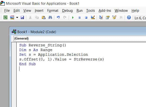
Sub Reverse_String()
Dim s As Range
Set s = Application.Selection
s.Offset(0, 1).Value = StrReverse(s)
End SubFollow these steps:
- From the Developer Menu Ribbon, select Visual Basic.
- Once your VBA window opens, Click Insert->Module. Now you can start coding. Type or copy-paste the above lines of code into the module window. Your code is now ready to run.

- Select a single cell containing the text you want to reverse. Make sure the cell horizontally next to it is blank because this is where the macro will display the reversed string.
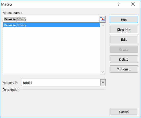
- Navigate to Developer->Macros->Reverse_String->Run.

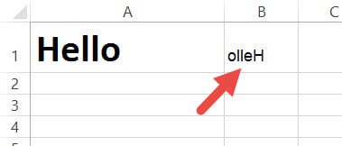
You will now see the reversed string next to your selected cell.
Note: If you can’t see the Developer ribbon, from the File menu, go to Options. Select Customize Ribbon and check the Developer option from the Main Tabs.
Finally, Click OK.
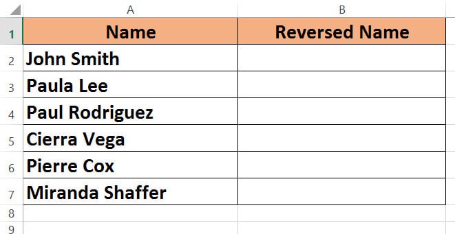
Reversing a List of Strings in Excel using VBScript
Using VBScript to reverse a long list of strings is easy too! Say you want to reverse the following set of names:
Here’s the VBA code that we will be using to reverse all strings in a column. Select and copy it.
Sub reverse_string_range()
Dim s As Range
Dim cell As Range
Set s = Application.Selection
i = 0
For Each cell In s
cell.Offset(0, 1).Value = StrReverse(cell)
i = i + 1
Next cell
End SubFollow these steps:
- From the Developer Menu Ribbon, select Visual Basic.
- Once your VBA window opens, Click Insert->Module. Now you can start coding. Type or copy-paste the above lines of code into the module window. Your code is now ready to run.
- Select the range of cells containing the text you want to reverse. Make sure the column next to it is blank because this is where the macro will display the reversed strings.
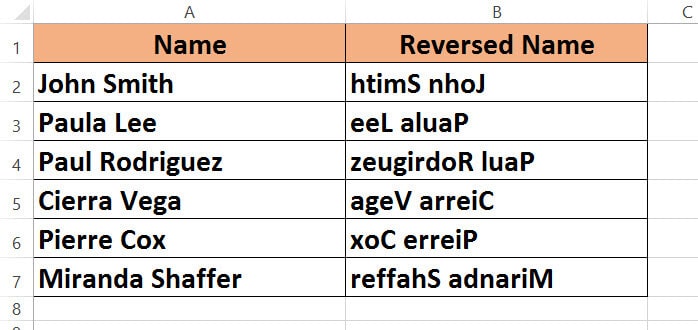
- Navigate to Developer->Macros->reverse_string_range->Run.
You will now see the reversed strings next to your selected range of cells.
Do remember to keep a backup of your sheet, because the results of VBA code are usually irreversible.
To wrap it up, we saw two ways to reverse strings in Excel. One method uses a formula and the other method uses VBA code.
The first method is alright if you don’t really feel comfortable working with VBA code. But it is beneficial only if you have one or a few cells that you want to reverse.
If there are more cells that need to be reversed, it can prove to be time-consuming.
Instead, you can use the second method (using VBA code), because it saves time and with just a few clicks, you can get a whole list of strings reversed in one go.
Although there are no straight ways to reverse a text string in Excel, I hope the methods shown here will help you get it done easily.
I hope you found this tutorial useful.
Other Excel tutorials you may find useful:
- How to Merge First and Last Name in Excel
- How to Split One Column into Multiple Columns in Excel
- How to Remove Commas in Excel (from Numbers or Text String)
- How to Generate Random Numbers in Excel (Without Duplicates)
- How to Add Text to the Beginning or End of all Cells in Excel
- How to Extract Number from Text in Excel (Beginning, End, or Middle)
- How to Change Uppercase to Lowercase in Excel
- How to Find the Last Space in Text String in Excel?
- Switch First and Last Name with Comma in Excel (Flip Names)