Get a List of All Sheet Names in Excel

You may want to list all sheet names in your Excel workbook, for instance, when creating a Table of Contents (TOC) for easy navigation across multiple sheets.

I will show you three methods for listing all sheet names in your Excel workbook.

Method #1: Using GET.WORKBOOK & TEXTAFTER Functions

In this method, we are going to use an old macro for a function called GET.WORKBOOK that gives us a list of all the worksheet names.

The issue here is that you cannot use this function in the worksheet. However, you can use it in Named Ranges, which can then be used in the worksheet.

Let me show you how it works.

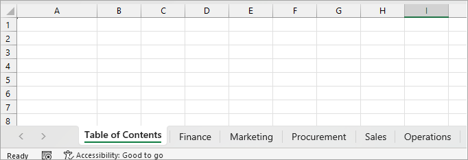
Let’s say you have a workbook with several sheets, shown in the example below.

In this workbook, I want to get the list of all the worksheet names.

Here’s how to do it:

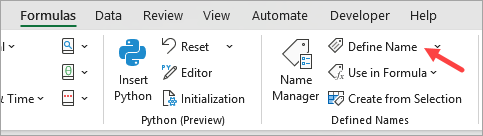
1. Open the Formulas tab and click on the Define Name drop-down on the Defined Names group.

The above step opens the New Name dialog box.

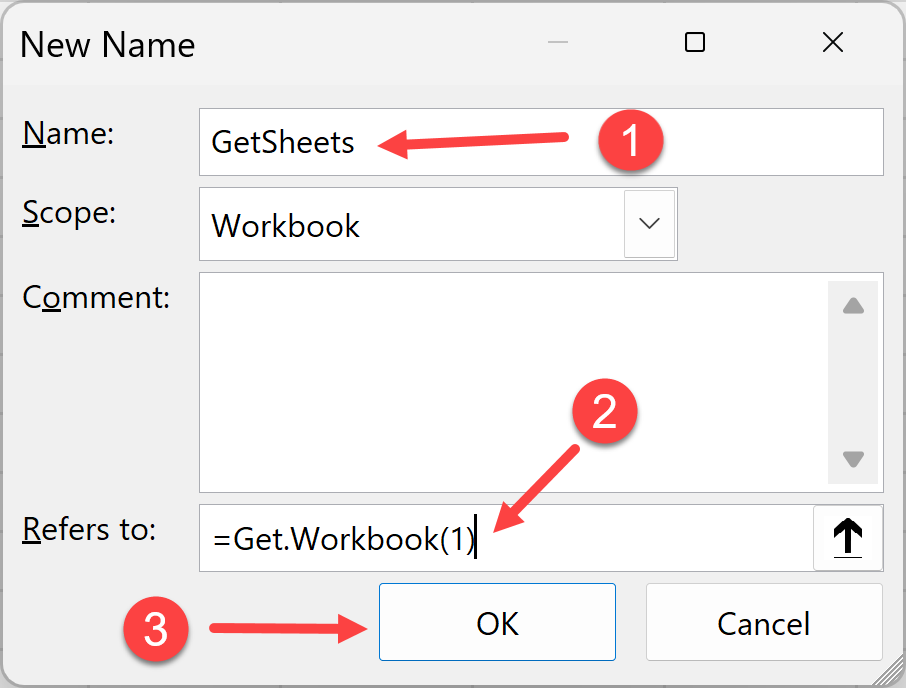
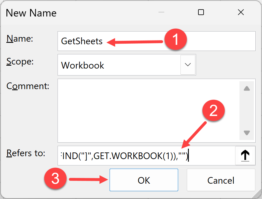
3. On the New Name dialog box, do the following:

• Enter ‘GetSheets’ in the Name box.
• Enter ‘=GET.WORKBOOK(1)’ in the ‘Refers to’ box.
• Click OK.

4. In cell A1, enter the following formula and hit Enter

=TEXTAFTER(TRANSPOSE(GetSheets),"]")

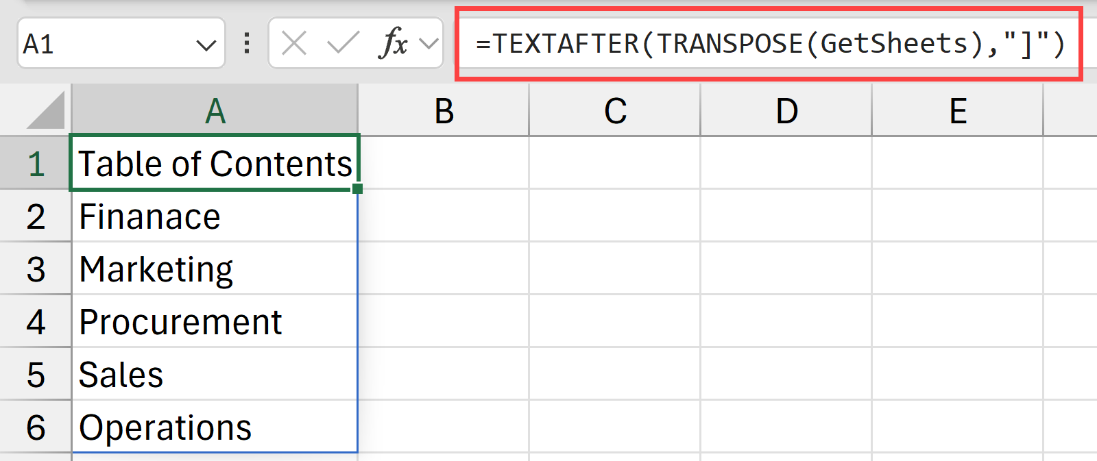
The above steps would give you all the sheet names in a column in the worksheet.

IMPORTANT: Since we are using an old Macro4 function, you need to ensure that you save this file as a macro-enabled file with a .XLSM extension. Otherwise, the formula would be lost when you save the file.

Explanation of the Formula

• The named range ‘GetSheets’ returns a horizontal array of sheet names, where there is the worksheet name before the sheet name as well (e.g., [Book1]Sheet1)
• TRANSPOSE(GetSheets) – The TRANSPOSE function turns the horizontal array of worksheet names into a vertical one.
• TEXTAFTER(…, “]”) – The TEXTAFTER function extracts the portion of the sheet name coming after the right square bracket (]). So, in the context of our example, in cell A1, =TEXTAFTER(TRANSPOSE(GetSheets),”]”) returns ‘Table of Contents.’

Note: While this formula isn’t dynamic, you can update the results after making changes to the sheets by clicking in the formula on the formula bar and pressing Enter. It would also update if you make any other changes in the worksheet or workbook.

Getting the #BLOCKED Error? Here is how to fix it!

If you encounter the #BLOCKED error when you enter the formula, here are the steps to fix it:

1. Click the File button.
2. Click ‘Info’ on the navigation panel on the left of the Backstage view and ‘Trust Center Settings’ on the right.

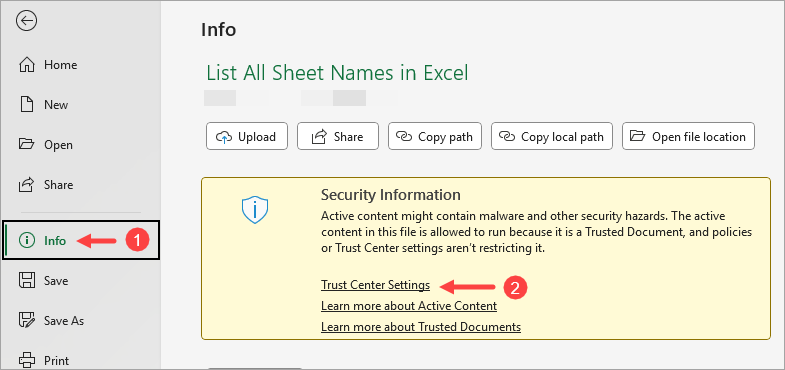
The above step opens the ‘Trust Center’ dialog box.

3. Click ‘Macro Settings’ on the navigation panel on the left of the ‘Trust Center’ dialog box and check the ‘Enable Excel 4.0 macros when VBA macros are enabled’ option on the right.

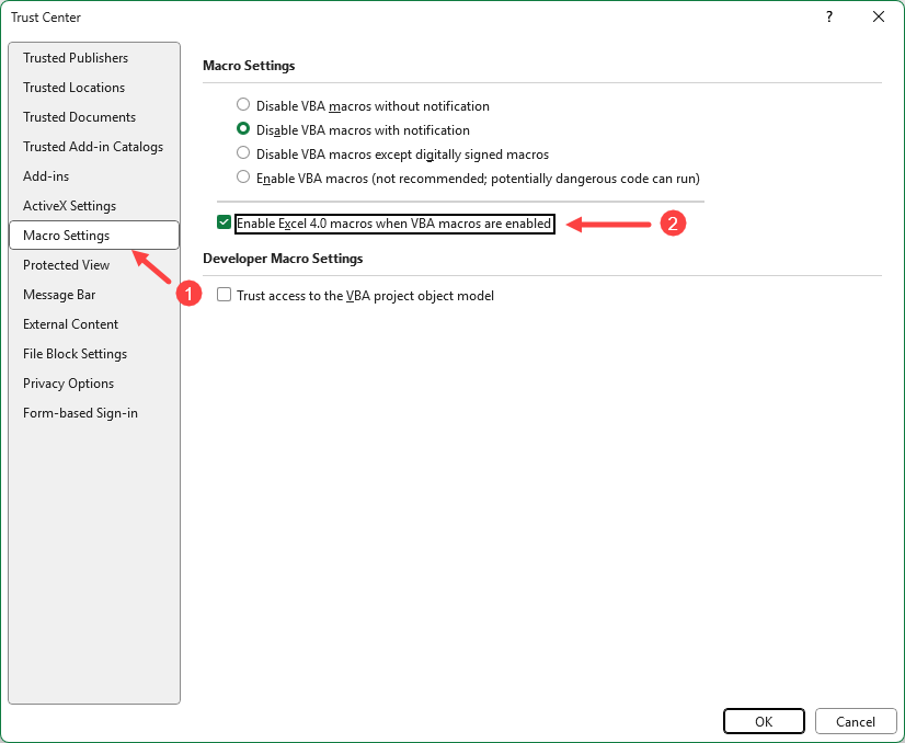
4. Click OK.
5. Restart Excel.

Also read: Get Current Sheet Name in Excel

Method #2: Using GET.WORKBOOK & INDEX Function (All Excel Versions)

If you have an older version of Excel and don’t have access to the newer functions, you can use an INDEX formula instead.

This method will work for all versions of Excel, but the drawback is that it will not give you the list of all the sheet names with a single formula. You will have to copy the formula for multiple cells to get all the sheet names.

Let’s say you have a workbook with several sheets, shown in the example below.

You can use an INDEX formula to create a list of all the sheets in the workbook in the ‘Table of Contents’ sheet.

Here’s how to do it:

1. Open the Formulas tab and click on the Define Name drop-down on the Defined Names group.

The above step opens the New Name dialog box.

3. On the New Name dialog box, do the following:

• Enter GetSheets in the Name box.
• In the Refers to field, enter the following formula.

=REPLACE(GET.WORKBOOK(1),1,FIND("]",GET.WORKBOOK(1)),"")

• Click OK

4. In cell A1, enter the following formula:

=INDEX(GetSheets, ROW())

4. Drag the fill handle to copy the formula down until you see the #REF! error.

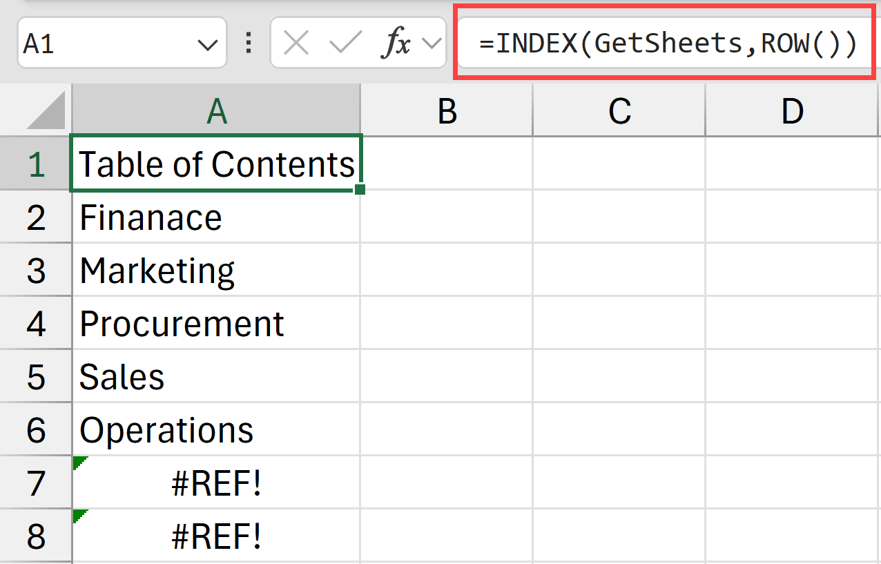
5. Remove all the #REF! errors, so you only have the sheet names.

Note: If you encounter the #BLOCKED error when you enter the formula, fix it as explained earlier in the section ‘How to Fix the #BLOCKED Error.’ 

Explanation of the Formula

There are two different formulas that I’ve used here:

1. In the name box to create the named range
2. In the worksheet

The formula below is used to create the named range:

=REPLACE(GET.WORKBOOK(1),1,FIND("]",GET.WORKBOOK(1)),"")

Here’s how it works:

• GET.WORKBOOK(1) – This macro 4.0 function returns all the sheet names in the target workbook, each prefixed with the workbook name in the format [Book1]Sheet1, [Book1]Sheet2, etc.
• FIND(“]”, GET.WORKBOOK(1)) – This segment of the formula finds the position of the closing square bracket (]), which marks the end of the workbook name.
• REPLACE(…, 1, FIND(…), “”) – Finally, the REPLACE function removes the workbook name and the last square bracket, leaving just the sheet name.

And then the following formula is used in the worksheet to get the list of all the sheet names

• The named formula ‘GetSheets’ returns an array of sheet names as explained in the previous section.
• The ROW() function returns the row number of the current cell. For instance, in cell A1, ROW() returns 1.
• INDEX(ListSheets, ROW()) – The INDEX function returns the Nth sheet name from the ‘GetSheets’ array. So, in the context of our example, in cell A1, =INDEX(GetSheets, 1) returns ‘Table of Contents.’

Method #3: Using Power Query

Suppose you have a workbook with several sheets, shown in the example below.

You can use Power Query to create a list of all the sheets in the workbook.

Here’s how to do it:

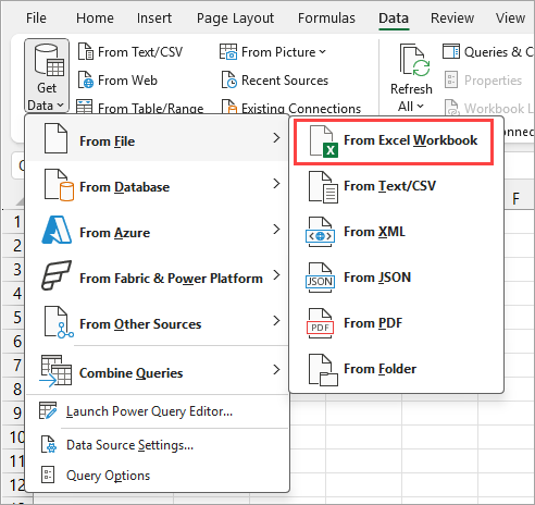
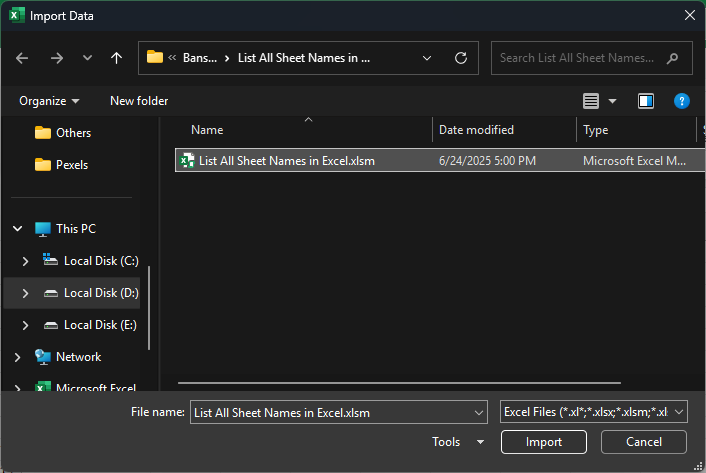
1. Click the Data tab, open the Get Data drop-down on the Get & Transform group, hover the mouse pointer over the From File option, and click the From Excel Workbook option on the submenu.

The above step opens the Import Data feature.

2. On the Import Data feature, navigate to where the target workbook is stored, select it, and click Import.

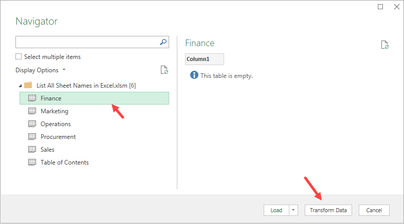
The above step opens Power Query’s Navigator feature.

3. On the Navigator feature, select any sheet on the navigation panel on the left and click the Transform Data command button on the right.

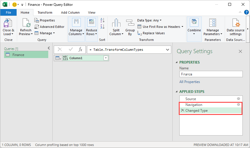
The above step opens the Power Query Editor.

4. On the Applied Steps section of the Query Settings panel, remove the Changed Type and Navigation steps by clicking the X icon beside them, and leave only the Source step.

The above step exposes the workbook’s metadata as shown below.

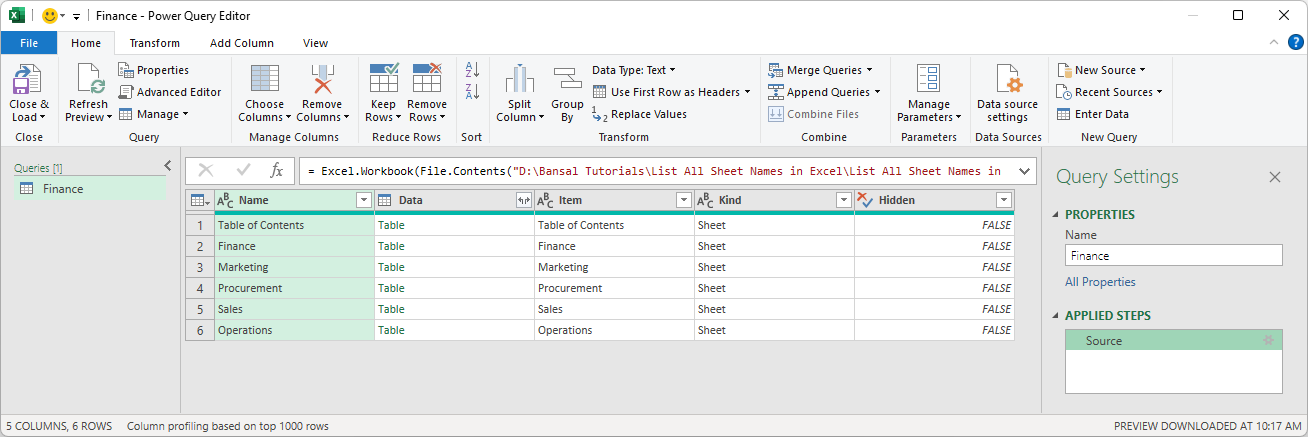
Note: Filter the ‘Kind’ column to show only ‘Sheet’ so that defined names and other non-sheet elements are excluded from the query results.

5. Right-click the header of the Name column and click the Remove Other Columns option on the shortcut menu.

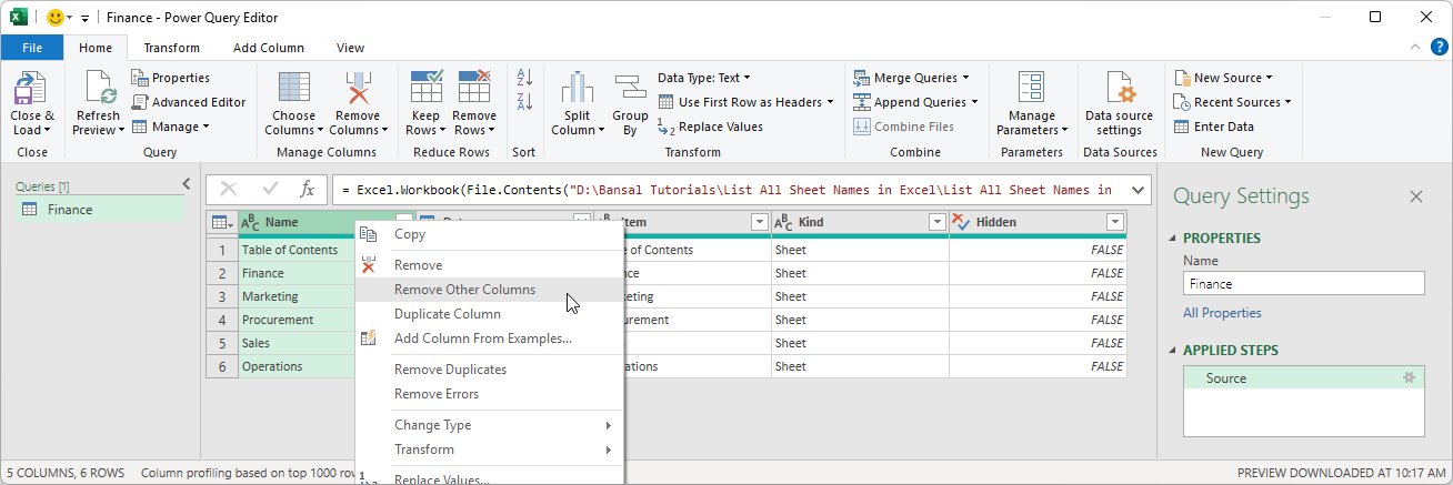
The above step removes all the other columns, leaving only the Name column.

6. Click the Close & Load command button on the Close group.

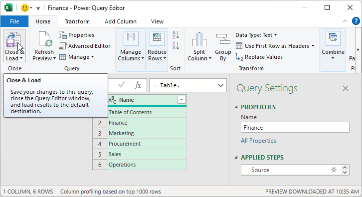
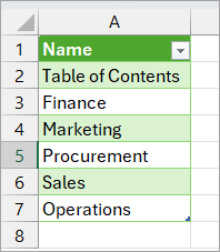
The above step loads a list of all sheet names in the workbook into a new worksheet.

Method #4: Using VBA Code

In this method, I’ll show you how to create a custom function using VBA that would instantly give you a list of all the sheet names in the current workbook.

Suppose you have a workbook with several sheets, shown in the example below.

Here are the steps to create the custom function using VBA and then use it in the worksheet

1. Open the VB Editor (you can use the keyboard shortcut Alt + F11, or you can go to the Developer tab and click on the Visual Basic icon)
2. In the VBA Editor, click on the Insert option and then click on Module. This will insert a new module where we are going to put our VBA code.
3. Copy the VBA code below into the newly inserted VBA module:

Function GetSheetNames(Optional ExcludeCurrent As Integer = 0) As Variant
    Dim ws As Worksheet
    Dim sheetNames() As String
    Dim i As Integer
    Dim currentSheetName As String
    Dim sheetCount As Integer
    
    ' Get the name of the sheet where the formula is being used
    currentSheetName = Application.Caller.Parent.Name
    
    ' Calculate how many sheets to include
    sheetCount = ThisWorkbook.Worksheets.Count
    If ExcludeCurrent = 1 Then
        sheetCount = sheetCount - 1
    End If
    
    ' Handle case where only one sheet exists and we're excluding it
    If sheetCount = 0 Then
        GetSheetNames = "No other sheets"
        Exit Function
    End If
    
    ' Initialize the array
    ReDim sheetNames(1 To sheetCount, 1 To 1)
    
    ' Loop through all worksheets and store their names
    i = 1
    For Each ws In ThisWorkbook.Worksheets
        ' Skip the current sheet if ExcludeCurrent = 1
        If ExcludeCurrent = 1 And ws.Name = currentSheetName Then
            ' Skip this sheet
        Else
            sheetNames(i, 1) = ws.Name
            i = i + 1
        End If
    Next ws
    
    ' Return the array of sheet names
    GetSheetNames = sheetNames
End Function

4. Close the VB Editor

With the above steps, we now have a custom function in our workbook (named GetSheetNames) that we can use in any of our worksheets.

Now, to use it in the workbook, go to any cell and enter the following formula:

=GetSheetNames()

The above formula would instantly give you all the sheet names as a list in the column.

In case you do not want to include the sheet of the current worksheet in which the folder is used, you can use the formula below instead.

=GetSheetNames(1)

Remember to save your file as a macro-enabled file with the .xlsm extension because it has a VBA code in it. If you do not save it as a macro-enabled file, your VBA code will be lost.

In this article, I’ve shown you four methods to get a list of all the sheet names in the current workbook in Excel. In most cases, the fastest way is to use the Get.Workbook function. However, in some cases, it may be more suitable to opt for the Power Query or VBA method.

Other Excel articles you may also like:

• How to Insert Sheet Name into Header or Footer in Excel?
• How to Remove Page Numbers in Excel