How to Get Sheet Names in Excel?

You may want to get the worksheet’s name while working with Excel.

For example, when creating a report that includes multiple worksheets, you may have the sheet name as a header or footer to help users navigate the report. 

Of course, you can manually type in the names, but the names will not automatically update if you rename the worksheets.

This tutorial shows four methods of getting the sheet name in Excel, and the name is automatically updated if it is changed. 

Method #1: Using TEXTAFTER and CELL Functions to Get the Worksheet Name in Excel

The TEXTAFTER function, only available in Excel 365, returns text that occurs after a given character or string. The CELL function returns information about a cell’s formatting, location, or contents.

We can use a formula that combines the two functions to get a worksheet name in Excel.

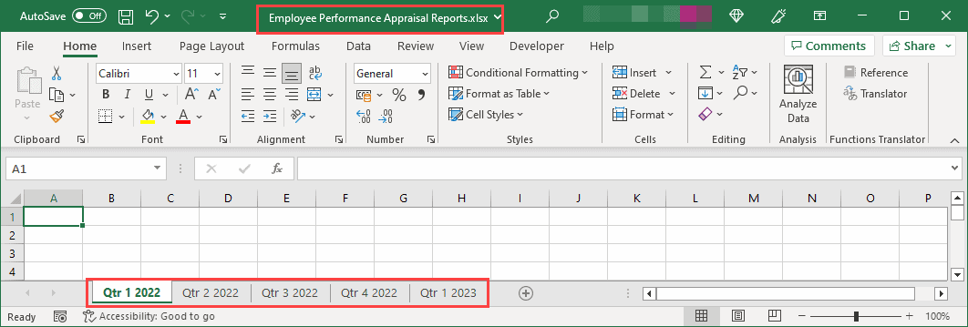
Let’s consider the following workbook, “Employee Performance Appraisal Reports,” which has five worksheets with different names:

We want to return the name of the current worksheet, “Qtr 1 2022”,  in a cell in the workbook using a formula that combines the TEXTAFTER and CELL functions.

We use the following steps:

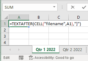
1. Select any cell in the active worksheet; in this case, we select cell A1 and enter the below formula:

=TEXTAFTER(CELL("filename",A1),"]")

Note: This formula only works if the workbook has been saved at least once. Otherwise, it returns the #N/A error because it cannot locate the workbook.

2. Press Enter.

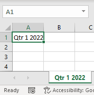
The name of the “Qtr 1 2022” worksheet is returned in cell A1 as shown below:

We get the respective worksheet names if we copy the formula to the other worksheets in the workbook.

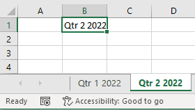
For example, when we copy the formula to cell B2 of the “Qtr 2 2022” worksheet, the worksheet’s name is returned in the cell as seen below:

Explanation of the formula

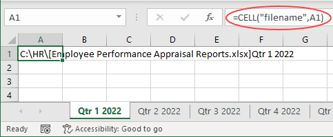
The CELL function’s info_type  argument is set to “filename,” and reference to cell A1 to return the full path to the active worksheet, as seen below:

The returned full path is then fed into the TEXTAFTER function as the text argument. The delimiter argument is set to “]” to extract only the text that is after the closing square bracket (“]”).

In our example, the result is “Qtr 1 2022”, the name of the active worksheet.

Also read: How to Get File Names from a Folder into Excel

Method #2: Use a Formula Combining MID, CELL, and FIND Functions to Get Sheet Name in Excel

Another easy way to get sheet names in Excel is by using a combination of MID, CELL, and FIND functions.

• The MID function returns the text string characters from inside a text string, given a starting position and length.
• The CELL function returns information about a cell’s formatting, location, or contents.
• The FIND function is case-sensitive and returns the starting position of one text string within another.

We can use a formula that combines the three functions to get a worksheet name in Excel.

We have the following workbook, “Employee Performance Appraisal Reports,” which has five worksheets with different names:

We want to return the name of the current worksheet, “Qtr 1 2022”,  in a cell in the workbook using a formula that combines the MID, CELL, and FIND functions.

We use the following steps:

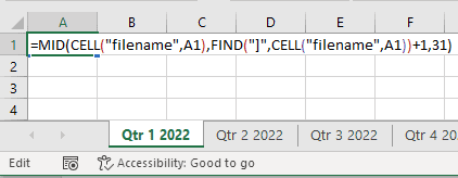
1. Select any cell in the current worksheet; in this example, we select cell A1 and enter the formula below:

=MID(CELL("filename",A1),FIND("]",CELL("filename",A1))+1,31)

Note: This formula will only work if the workbook has been saved at least once. Otherwise, the formula returns the #VALUE! error because it cannot locate the workbook.

2. Press Enter.

The current worksheet’s name is returned in cell A1 as seen below:

If we copy the formula to any cell in the other worksheets, the worksheet’s respective name is displayed in the selected cell.

Let’s, for example, copy the formula to cell G1 of the “Qtr 1 2023” worksheet:

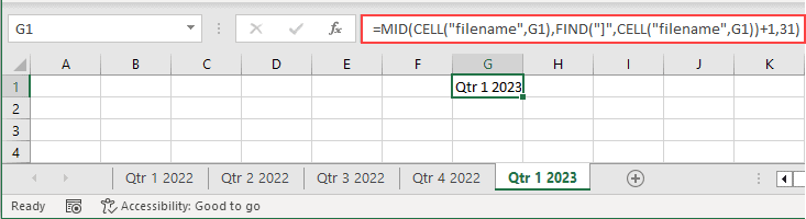
The formula returns the name of the worksheet in cell G1.

Explanation of the formula 

=MID(CELL(“filename”,A1),FIND(“]”,CELL(“filename”,A1))+1,31)

• CELL(“filename”,A1) – The first CELL function’s info_type argument is set to “filename” and reference argument to cell A1 to return the full path to the active worksheet as shown below:

The full path to the worksheet is passed to the MID function as the text argument.

• FIND(“]”,CELL(“filename”,A1))+1 – The FIND function returns the position of the closing square bracket in the full path. The position is increased by 1 to calculate the starting position of the worksheet name. The computed result is passed to the MID function as the start_num argument.
• Finally, the value 31, the maximum number of characters allowed in a worksheet name, is passed to the MID function as the num_chars argument. The value ensures that the MID function extracts the full worksheet name to the right of the closing square bracket. The final result in our example is “Qtr 1 2022,” the name of the current worksheet. 

Method #3: Using RIGHT, CELL, LEN, and FIND Functions to Get the Worksheet Name in Excel

The RIGHT function returns the specified number of text string characters from the end of a text string. The CELL function returns information about a cell’s formatting, location, or contents. The LEN function returns the number of characters in a text string, and the FIND function, which is case-sensitive, returns the starting position of one text string within another. 

We can apply a formula combining the four functions to get the name of a worksheet in Excel.

Assume we are working on the following “Employee Performance Appraisal Reports” workbook that has five worksheets with different names:

We want to use a formula combining the RIGHT, CELL, LEN, and FIND functions to return the name of the active worksheet, “Qtr 1 2022,” in a cell in the workbook.

We proceed as follows:

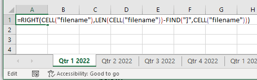
1. Select any cell in the active worksheet; in this example, we select cell A1 and enter the formula below:

=RIGHT(CELL("filename"),LEN(CELL("filename"))-FIND("]",CELL("filename")))

Note: This formula only works if the workbook is saved at least once. Otherwise, the formula returns the #VALUE! error because it cannot find the workbook.

2. Press Enter.

The name of the active worksheet is displayed in cell A1:

If we copy the formula to any cell in the other worksheets, the worksheet’s respective name is returned in the selected cell.

Let’s, for example, copy the formula to cell E2 of the “Qtr 3 2022” worksheet:

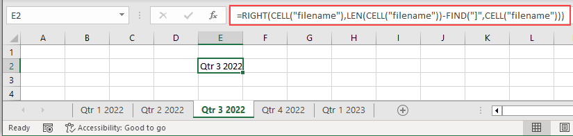
The name of the active worksheet is shown in cell E2.

Explanation of the formula 

=RIGHT(CELL(“filename”),LEN(CELL(“filename”))-FIND(“]”,CELL(“filename”)))

• CELL(“filename”) The first CELL function returns the full path to the active worksheet as shown below:

The worksheet’s path is then passed to the RIGHT function as the text argument.

• LEN(CELL(“filename”) The LEN function returns the number of characters in the active worksheet’s full path text string.
• FIND(“]”,CELL(“filename”)) The FIND function returns the position of the closing square bracket in the full path text string. 
• LEN(CELL(“filename”))-FIND(“]”,CELL(“filename”)) The number returned by the FIND function is subtracted from the entire length of the full path text string returned by the LEN function. The result is the length of the name of the active worksheet. The result is passed to the RIGHT function as the num_chars argument.
• Finally, the RIGHT function utilizes the text, and the num_chars values passed to it to extract the name of the current worksheet. 

Appending Text to the Worksheet Name

If printing a report that includes many worksheets, we could add more descriptive text to the worksheet name to help users quickly navigate the information. 

For example, if we have a worksheet name “Qtr 1 2022,” we may want to add the text “Employee Performance Appraisal Report for” to the name so that the report’s title reads “Employee Performance Appraisal Report for Qtr 1 2022.”

We can achieve this by joining the formulas we have already described to the additional text we want using the ampersand (&) operator.

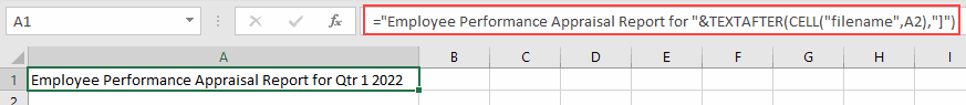
For example, the formula below adds the text “Employee Performance Appraisal Report for” to the worksheet name:

="Employee Performance Appraisal Report for "&TEXTAFTER(CELL("filename",A2),"]")

We can also use the CONCAT function as in the example below:

How to List All Worksheet Names in a Workbook Using a Formula

We may want a list of all worksheet names in a workbook.

Suppose we have the following “Employee Performance Appraisal Reports” workbook with a Summary worksheet and five other worksheets.

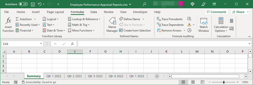
We want to use a formula to extract a list of the worksheets’ names in the “Summary” worksheet of the workbook. 

We use the following steps:

1. Select any cell in the Summary worksheet; we select cell A1 in this example.
2. On the Formulas tab, on the Defined Names group, click the Define Name button.
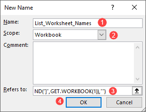
3. On the New Name dialog group that pops up, do the following:

• On the Name box, type “List_Worksheet_Names.” Remember, the name should not have spaces.
• Open the Scope drop-down list and select Workbook.
• Type the formula “=REPLACE(GET.WORKBOOK(1),1,FIND(“]”,GET.WORKBOOK(1)),””)” on the Refers to box and click OK.

Note: The GET.WORKBOOK function is an Excel 4.0 function that cannot be used directly in cells but works with named ranges.

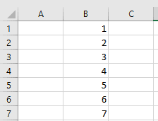
4. Enter the values 1 to 7 in the cell range B1:B7 as shown below:

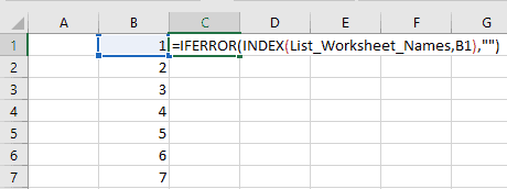
5. Select cell C1 and enter the formula below:

=IFERROR(INDEX(List_Worksheet_Names,B1),"")

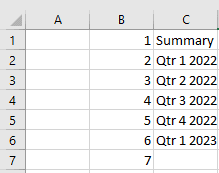
6. Drag the Fill Handle to copy the formula down the column to get the following list of names of worksheets in the workbook:

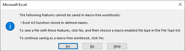
7. Save the workbook as a Macro-Enabled Workbook (*.xlsm), so you do not lose the list. Excel informs you accordingly if you attempt to save the workbook as a regular (*.xlsx) file.

Explanation of the technique

• The formula REPLACE(GET.WORKBOOK(1),1,FIND(“]”,GET.WORKBOOK(1)),””) replaces all the characters in each worksheet’s full path text string up to and including the closing square bracket with empty strings leaving only the worksheet name. This formula effectively generates an array of the names of the worksheets in the workbook.
• INDEX(List_Worksheet_Names,B1) The INDEX function uses the value in cell B1, in this case, one (1), to return the first worksheet name in the array. As the formula is copied to the other cells, it returns the second and third worksheet names, and so on.
• The IFERROR function that wraps the formula returns an empty string after all the worksheet names in the array have been listed.

Some Use Cases where Getting Sheet Names Could Be Useful

Knowing how to get sheet names in Excel can be useful in many different situations.

Here are some use cases where I have found it useful to quickly know the name of the current sheet name or all sheet names in the file.

1. When Consolidating Data From Multiple Excel Files

When you have multiple Excel files with similar data structures, you may want to consolidate them into a single file.

In this case, knowing the sheet names can help you easily identify which sheets contain the data you need to consolidate.

You can then use formulas or VBA code to extract the data from multiple sheets and combine them into one single sheet or file.

2. When Automating Reports

If you regularly create reports that involve multiple sheets, knowing how to get sheet names can save you time and effort.

For example, you can use VBA code to loop through all the sheets in a workbook and extract data from all the sheets or specific sheets with specific sheet names (such as the year number of department name).

You can also use sheet names to dynamically reference cells or ranges in your formulas or VBA code.

3. Finding Missing Data/Sheet

If you’re collating data and combining different sheets into one Excel file, getting a list of all the sheet names can help you spot if there are any missing sheets that needs to be added.

Getting all the sheet names in a column then can be very useful in such a situation.

4. Data Validation

When creating data validation rules in Excel, you may want to restrict the input to a specific range of cells on a particular sheet.

Knowing the sheet name can help you easily specify the range of cells you want to restrict the input to. This can help prevent errors and ensure data consistency.

5. Collaborating with Others

If you are collaborating with others on an Excel workbook, knowing the sheet names can help you communicate more effectively.

For example, you can refer to specific sheets by name when discussing the data or formulas with your colleagues.

This can help ensure everyone is on the same page and minimize confusion.

This tutorial showed four techniques for getting worksheet names in Excel. We hope you found the tutorial helpful.

Other Excel articles you may also like:

• Add New Sheet in Excel (Shortcut)
• Switch Between Tabs/Worksheets in Excel (Shortcut)
• 3 Easy Ways to Duplicate Sheet in Excel (Shortcuts + VBA)