When printing out an Excel worksheet, we usually just need to see the data. We don’t really care much for the location of the data, neither do we want to know which row the data belongs to.
That’s why Excel generally omits the row numbers and column letters when we print a worksheet.
There may be times, however, when we want to print the row numbers, as a sort of reference to quickly guide the reader to an important bit of data.
In this tutorial we will see three ways in which you can print row numbers in Excel:
- Using the Page Setup dialog box
- Using the Page Layout tab
- Using the ROW() function
The first two methods will result in both the row number and column letter appearing in the printout, while the third method lets you display just the row numbers, without having to print the column letters.
Throughout this tutorial, we will try to print the following sheet, along with row numbers for each row of cells:

For simplicity, we kept the dataset small. Let’s take a look at each of the above methods one by one.
Method 1: Print Row Numbers Using the Page Setup Dialog Box
The Page Setup dialog box lets you adjust all your print and layout settings from a single place. So this is a great place from where you can set your printouts to contain row numbers and column letters.
Unfortunately, you will need to print both row numbers and column headers using this method. It doesn’t give you the option to print either one.
Here’s how you can print both row numbers and column headers using the Page Setup dialog box:
- Make sure your worksheet is ready for printing.
- Press CTRL+P (if you’re on a Mac, press Cmd+P), or navigate to File->Print. This will bring you to Print Preview mode

- On the left-hand side, you will see a list of options (drop-down menus) under Settings. Just below these setting options, you will see a link that says ‘Page Setup’.

- Click on the Page Setup link. This will open the Page Setup dialog box.
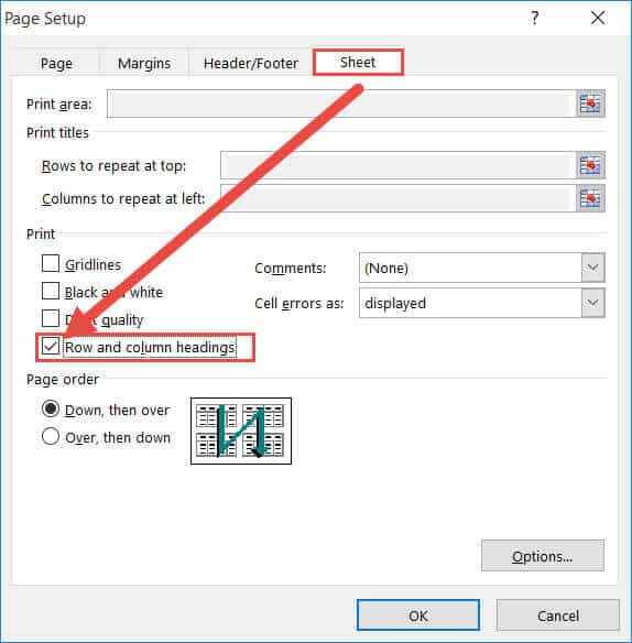
- Click on the Sheet tab in the dialog box.
- Under the Print section, you will find four checkboxes. Make sure the checkbox next to ‘Row and Column headings’ is checked.

- Click OK to close the Page Setup dialog box.
- This will bring you back to the Print Preview mode.
- You should be able to now see the row numbers and column letters in the print preview.

- If everything is alright, click the Print button to start printing.


Note: There are other ways to get to the Page Setup dialog box. For example, you can open it using the Dialog Box Launcher (a small tilted arrow) for the Page Setup group. This comes under the Page Layout tab of your Excel window.

Also read: How To Make Excel Spreadsheet Bigger When Printing
Method 2: Print Row Numbers Using the Page Layout Tab
You can also get Excel to print row numbers directly from the Page Layout tab itself. The Page Layout tab contains all options that let you arrange your printouts just the way you want. Using this tab, you can set margins, apply themes, control page orientation, and set gridlines and headings.
Here’s how you can print row numbers and column headers using Excel’s Page Layout tab:
- Make sure your worksheet is ready for printing.
- Click on the Page Layout tab from the Excel window. Alternatively, you can use the shortcut ALT+P to select the Page Layout tab.
- Under the Sheet Options group, you will see two categories: Gridlines and Headings.

- Under the Headings category, make sure the checkbox next to ‘Print’ is checked.

- This will make sure your printout contains the row and column headings for each cell.
- You can now go ahead and check the print preview by pressing the shortcut CTRL+P on the keyboard (Cmd+P if you’re on a Mac).
- If everything is alright, click the Print button to start printing.


Note: This method lets you include both row numbers and column headers in your printout. Just like method 1, you cannot set it to print just the row numbers. The column header also gets printed along with it by default.
Also read: How to Make Excel Columns the Same Width
Method 3: Print Row Numbers Using the ROW() Function
The first two methods are great if you are alright with getting columns headers along with row numbers in the printout.
If you want just the row numbers, not the column headers, then there’s, unfortunately, no menu option for this in Excel. However, there is a way around this, and that is by using the ROW() function.
The ROW function is a built-in function in Excel that returns the row number for a particular cell.
When you enter just the ROW function without any parameters in the parentheses, then it returns the row number for the cell that it is entered into.
If instead, you include a cell reference into the parentheses, then it returns the row number for that particular cell reference.

This means ROW(A1) returns 1 because it belongs to the first row. Similarly, ROW(A6) returns 6 because it belongs to the 6th row.

Similarly, if you put just =ROW() in cell A1, it will also return 1 and if you put it in row A6, it will return 6.
Now let us see how you can use the ROW() function to print row numbers in your sheet:
- Insert an extra column to the left of the first column of your sheet (by right-clicking on the first column header and clicking insert from the popup menu that appears).

- Type =ROW() in the first cell of the first row (cell A1).
- Drag down the fill handle (located at the bottom right corner) of this cell till the last row of your data.
- This will copy the formula to all the rows containing data. You now have row numbers for all data.

- Format the new column (A) to appear in your desired format. For example, add borders, font styling, background colors, or whatever you need.
- Make sure your worksheet is ready for printing.

- You can now go ahead and check the print preview by pressing the shortcut CTRL+P on the keyboard (Cmd+P if you’re on a Mac).
- If everything is alright, click the Print button to start printing.


In this tutorial, we showed you three ways to print row numbers along with your data in Excel. The first two methods are good if you want to print both row and column headers.
However, if you want to avoid printing the column headers, then you can go for Method 3. We hope this was helpful to you.
Other Excel tutorials you may like:
- How to Fit to Page in Excel (Print on One Sheet)
- How to Print Multiple Tabs/Sheets in Excel
- Get File Names from a Folder into Excel (Copy Files Names to Excel)
- How to Set a Row to Print on Every Page in Excel
- How to Save Selection in Excel as PDF
- How to Change Page Orientation in Excel (for Printing)
- How to Enter Sequential Numbers in Excel?
- How to Print Comments in Excel?
- Get a List of All Sheet Names in Excel
Method 3: Print Row Numbers Using the ROW() Function
I actually got this to work. I am so happy. However, I actually need Row 2 to be Row 1 and Row 3 to be Row 2, etc.
My Row 1 is the headings, and I don’t want to count that in my total number.
use =ROW()-1 in box row 2 A and drag it to the last row