OFFSET Function in Excel

If you want to grab a cell or a range of cells that sits a certain number of rows and columns away from a starting point, the OFFSET function in Excel is built for that.

It can also return a resized range, which is what makes it useful for dynamic sums, last-N calculations, and charts where the data keeps growing.

One thing to know up front: OFFSET is a volatile function, so it recalculates every time anything in the workbook changes.

OFFSET Function Syntax

Here is the syntax of the OFFSET function:

=OFFSET(reference, rows, cols, [height], [width])

• reference – The starting cell or range that the offset is measured from.
• rows – The number of rows to move from the reference. Positive moves down, negative moves up.
• cols – The number of columns to move from the reference. Positive moves right, negative moves left.
• height – Optional. The height (in rows) of the returned range. Defaults to the height of the reference.
• width – Optional. The width (in columns) of the returned range. Defaults to the width of the reference.

When to Use the OFFSET Function in Excel

Use this function when you need to:

• Build a range that resizes as your data grows (dynamic sums, averages, or chart sources).
• Pull a value from a position that depends on a count or a row number returned by another formula.
• Combine with MATCH to do a two-way lookup based on row and column labels.
• Return the last N rows of a list, no matter how many rows the list has today.

Let me show you a few practical examples of how to use this function.

Example 1: Basic OFFSET Navigation

Let’s start with the simplest case. The whole point here is to see how the rows and cols arguments shift the reference.

Below is a small dataset with quarterly sales for eight products. The reference cell B2 holds Laptop’s Q1 sales value.

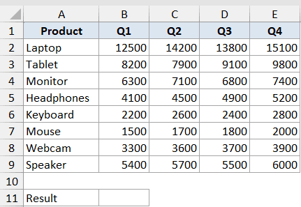
I want to return the Q3 sales value for “Headphones” using OFFSET starting from B2.

Here is the formula:

=OFFSET(B2, 3, 2)

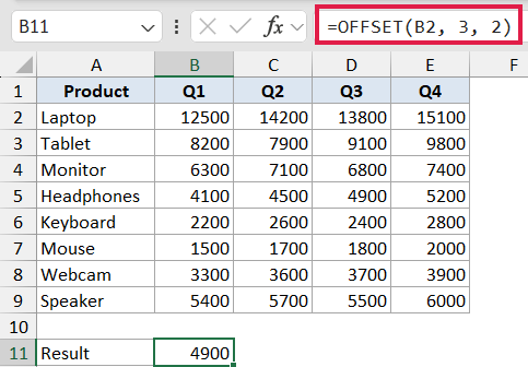
In the above formula, B2 is the starting cell. The rows argument is 3, so OFFSET moves down 3 rows to row 5 (Headphones). The cols argument is 2, so it then moves 2 columns to the right, landing on the Q3 column. The result is 4900.

The height and width arguments are left blank, so OFFSET returns a single cell that matches the size of the reference (B2 is one cell, so the result is one cell).

Example 2: Dynamic Sum for a Growing List

Here’s a scenario where OFFSET earns its keep.

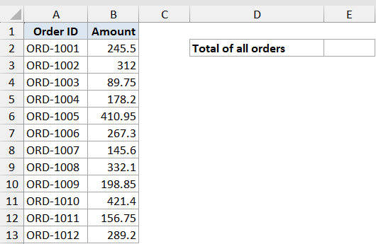
You have a list of daily order amounts in column B that keeps growing as new orders come in, and you want a running total that always covers the whole list, no matter how many rows it has.

Below is the dataset. Column A has order IDs, column B has the order amount, and the “Total of all orders” cell sits in E2 with the label in D2.

Here is the formula in cell E2:

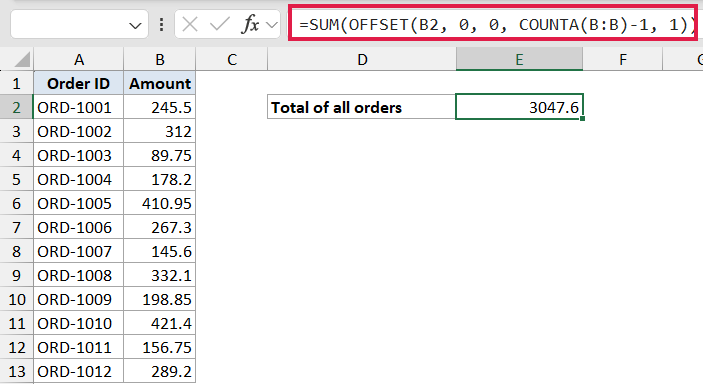
=SUM(OFFSET(B2, 0, 0, COUNTA(B:B)-1, 1))

How this formula works:

• B2 is the starting cell (first order amount).
• rows and cols are both 0, so OFFSET doesn’t move from B2.
• height is COUNTA(B:B)-1, which counts every non-empty cell in column B and subtracts 1 for the header. That’s how many rows the returned range covers.
• width is 1, so the range stays one column wide.
• SUM then adds up everything in that resized range.

When a new order is added in column B, COUNTA picks it up, the OFFSET range grows by one row, and SUM updates automatically.

In Excel 365 you can skip OFFSET entirely. Convert the list to a Table and write =SUM(Orders[Amount]). The Table reference auto-expands, isn’t volatile, and recalculates much less often.

The OFFSET version still works everywhere, but reach for Tables first on modern Excel.

Example 3: Last N Rows of a List

This one shows OFFSET pulling out the most recent entries. Useful for things like a “last 5 transactions” tile on a dashboard.

Same rule as Example 2: keep the formula outside the column the OFFSET reads from. The COUNTA on column B would otherwise loop back on itself.

Below is a list of transaction amounts in column B (rows 2 onwards). The “Sum of last 5” cell sits in E2 with the label in D2.

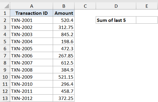
Here is the formula in cell D2:

=SUM(OFFSET(B1, COUNTA(B:B)-5, 0, 5, 1))

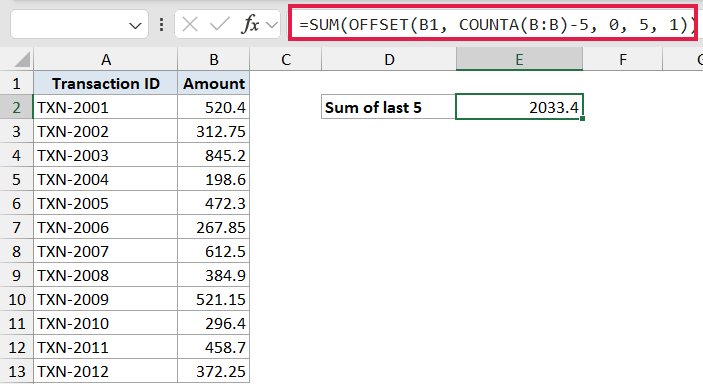
How this formula works:

• B1 is the starting cell (the header row).
• rows is COUNTA(B:B)-5. COUNTA gives the count of filled cells in column B, and subtracting 5 jumps us to the row that’s 5 from the bottom.
• cols is 0, so we stay in column B.
• height is 5, so the returned range is 5 rows tall starting from that jump-off row.
• width is 1.

SUM then totals just those last 5 cells.

In Excel 365, =SUM(TAKE(B2:B1000, -5)) does the same job without volatility. TAKE with a negative number pulls from the bottom. Same idea, cleaner formula.

Pro Tip: This pattern works for AVERAGE, MAX, MIN, and any other function that takes a range. Just swap SUM for the function you need.

Example 4: Two-Way Lookup with OFFSET and MATCH

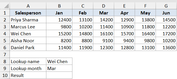
This is the classic OFFSET combo. You have a table with row labels on the left and column labels on top, and you want to pull a value where a specific row meets a specific column.

Below is a small table of monthly sales by salesperson. Names are in column A (A2:A6), months are in row 1 (B1:G1), and the sales values fill the grid in between. The lookup card sits below the data: name in B8, month in B9, result in B10.

Here is the formula in cell B10:

=OFFSET(A1, MATCH(B8, A2:A6, 0), MATCH(B9, B1:G1, 0))

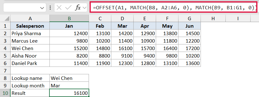
How this formula works:

• A1 is the anchor (the top-left corner of the table).
• The first MATCH finds the row position of the salesperson name inside A2:A6. If the name is the third one in the list, MATCH returns 3, so OFFSET moves down 3 rows.
• The second MATCH finds the column position of the month inside B1:G1. If the month is the third column, MATCH returns 3, so OFFSET moves 3 columns to the right.
• With both height and width left out, OFFSET returns a single cell at the intersection.

In Excel 365, you can do the same two-way lookup with XLOOKUP and skip the volatile OFFSET entirely: =XLOOKUP(B8, A2:A6, XLOOKUP(B9, B1:G1, B2:G6)).

If you have INDEX/MATCH muscle memory, =INDEX(B2:G6, MATCH(B8, A2:A6, 0), MATCH(B9, B1:G1, 0)) is also non-volatile and works in every modern version of Excel. The OFFSET version still works, but INDEX or XLOOKUP is the better long-term habit.

Example 5: Resized Range with Height and Width

The height and width arguments are where OFFSET earns its name as more than just a navigation helper. Hand it a height bigger than 1 and it returns a multi-cell range, ready to feed into SUM, AVERAGE, COUNT, or any other function that takes a range.

Below is a list of monthly revenue values in column B (B2:B13). The result cell sits in E2 with the label in D2.

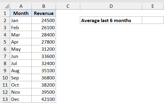
I want the average revenue for the second half of the year (July through December). Here is the formula in cell E2:

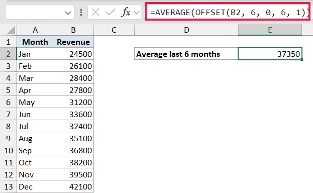
=AVERAGE(OFFSET(B2, 6, 0, 6, 1))

How this formula works:

• B2 is the starting cell (January’s revenue).
• rows is 6, so OFFSET moves 6 rows down to B8 (July).
• cols is 0, so we stay in column B.
• height is 6, so the returned range is 6 rows tall (B8:B13, July through December).
• width is 1.

AVERAGE then computes the mean of those six values.

This pattern is the building block for OFFSET-based dynamic ranges. Swap the literal 6 for COUNTA(B:B)-1 and the height resizes automatically as new months are added. That’s the expression you’d paste into a named range (Formulas > Define Name) for a chart whose source grows over time.

The named-range definition uses the OFFSET formula inside the “Refers to” box, not inside a worksheet cell, which is what keeps it out of column B and free of circular references.

In Excel 365, the simpler way for the “growing range” case is to convert the data to a Table (Ctrl+T) and build the chart from the Table. The Table auto-expands as you add rows, no named range or OFFSET needed, and there’s no volatility hit.

Tips & Common Mistakes

• OFFSET is volatile. It recalculates every time anything in the workbook changes, even cells it doesn’t depend on. A handful of OFFSET formulas is fine. Hundreds of them in a large workbook can make Excel noticeably sluggish. INDEX is a non-volatile drop-in for many OFFSET use cases, so prefer INDEX where you have a choice.
• Circular references: If your OFFSET formula uses COUNTA(B:B) and the formula itself sits in column B, Excel flags it as circular because the formula’s range includes itself. Put the formula in a different column (D or beyond), or use a fixed range like B2:B1000 if you know the upper bound.
• #REF! errors: If the rows or cols argument pushes the result off the worksheet (negative rows past row 1, for example), OFFSET returns #REF!. Double-check that your offsets keep you inside the sheet.
• The reference doesn’t move; the result does. OFFSET doesn’t change the underlying reference, it just returns a different cell or range based on it. Wrap it in SUM, AVERAGE, MATCH, or any other function that accepts a range.
• Use COUNTA carefully: COUNTA(B:B) counts every non-empty cell in column B, including headers and stray text. Subtract the right number for your layout, and avoid using it if there are gaps in the column.
• Modern alternatives: On Excel 365, Excel Tables handle most “growing range” cases without OFFSET. TAKE, CHOOSEROWS, FILTER, and XLOOKUP cover the rest. The OFFSET patterns above are still worth knowing for older Excel versions and inherited workbooks.
• Spill behavior: When OFFSET returns a multi-cell range and the formula sits on a worksheet (not inside another function), it spills into the cells below in Excel 365. If the cells next to it are occupied, you’ll see a #SPILL! error.

That covers the main ways OFFSET gets used in real spreadsheets, from a simple cell shift to dynamic sums, two-way lookups, and resized ranges.

OFFSET is one of those functions that’s worth understanding even if you mostly reach for Tables or INDEX in your own work, because you’ll run into OFFSET in workbooks built by other people all the time.

Just keep the volatility cost in mind and prefer the non-volatile alternatives whenever you have the choice.

List of All Excel Functions