If you want a quick way to check whether a cell holds a number or something else, the ISNUMBER function is what you need.
It returns TRUE when the value is a number and FALSE for anything else, including text, errors, and blank cells. Dates and times count as numbers under the hood, so ISNUMBER returns TRUE for them too.
In this article, I’ll show you how ISNUMBER works with a few practical examples.
ISNUMBER Function Syntax in Excel
Here is the syntax of the ISNUMBER function:
=ISNUMBER(value)
- value – The value you want to check. This can be a cell reference, a range, a literal number, or a formula result. ISNUMBER returns TRUE if the value is a number, and FALSE for text, logical values, errors, or blank cells.
A small thing worth knowing. Numbers stored as text (often pasted in from other systems with a leading apostrophe) return FALSE, because Excel sees them as text strings. Dates return TRUE since dates are really numbers under the hood.
When to Use ISNUMBER Function
Use this function when you need to:
- Flag cells that contain numbers in a mixed list of values
- Check if a cell contains a specific substring by pairing it with SEARCH or FIND
- Build an IF formula that branches based on whether the input is a number
- Pull only the numeric entries out of a column using FILTER
- Count how many numeric values are in a range
Let me show you a few practical examples of how to use ISNUMBER.
Example 1: Check a Mixed List for Numbers
Let’s start with a simple example to see ISNUMBER in its most basic form.
Below is the dataset. I have a column of inventory entries in column A. Some are item names, some are quantities, and one was pasted in from another system as a text-stored number.
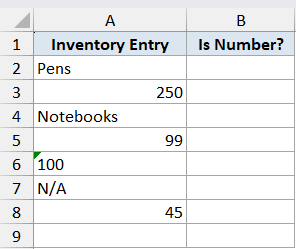
I want a TRUE or FALSE next to each value so I can see at a glance which entries are actual numbers.
Here is the formula:
=ISNUMBER(A2:A9)
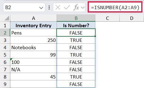
In the above formula, I’m feeding ISNUMBER the entire range A2:A9 in one shot. Since ISNUMBER spills in Excel 365, you only need to type the formula once in cell B2 and the results fill down to B9 automatically.
The quantities like 250, 99, and 45 return TRUE. Text entries like Pens and Notebooks return FALSE. The “100” that was pasted in as text also returns FALSE, since Excel sees it as a text string, not a number. The blank cell at the end returns FALSE too.
Pro Tip: If you are on an older version of Excel that does not support dynamic arrays, type =ISNUMBER(A2) in B2 and drag it down through B9. Same result, just the legacy way of doing it.
Example 2: Check if a Cell Contains Specific Text
Here’s where ISNUMBER really earns its keep.
Pairing ISNUMBER with SEARCH is the standard way to check whether a cell contains a specific piece of text. SEARCH returns the position of the substring when it finds one, and an error when it doesn’t. ISNUMBER turns that into a clean TRUE or FALSE.
Below is the dataset. I have a column of order references in column A. I want to flag the ones that contain “ORD” anywhere in the text.
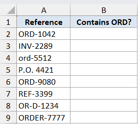
I want a TRUE or FALSE next to each reference based on whether “ORD” appears in it.
Here is the formula:
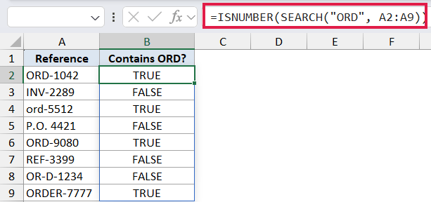
=ISNUMBER(SEARCH("ORD", A2:A9))
How this formula works:
- SEARCH looks for “ORD” inside each value in A2:A9. When it finds the substring, it returns the starting position as a number. When it doesn’t, it returns a #VALUE! error.
- ISNUMBER wraps that result. A number means SEARCH found a match, so ISNUMBER returns TRUE. An error means no match, so ISNUMBER returns FALSE.
Notice that “ord-5512” returns TRUE even though it’s lowercase. That’s because SEARCH is case-insensitive. “OR-D-1234” returns FALSE because the dash between OR and D breaks the substring, so SEARCH can’t find “ORD” as a continuous string.
Pro Tip: If you need a case-sensitive match, swap SEARCH for FIND. FIND works the same way but cares about case, so =ISNUMBER(FIND("ORD", A2:A9)) would treat “ord-5512” as a non-match.
Example 3: Label Each Row with IF and ISNUMBER
Here’s another practical scenario.
Sometimes a TRUE or FALSE isn’t quite what you need. You want a more descriptive label that tells you what kind of value sits in each row. Wrapping ISNUMBER in IF lets you do that in a single formula.
Below is the dataset. I have a column of survey responses in column A. Some respondents typed in a numeric score, others wrote a text answer.
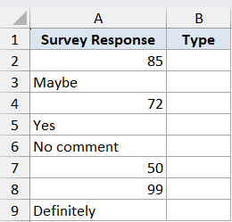
I want each row labeled as either Numeric or Non-numeric based on what’s in column A.
Here is the formula:
=IF(ISNUMBER(A2:A9), "Numeric", "Non-numeric")
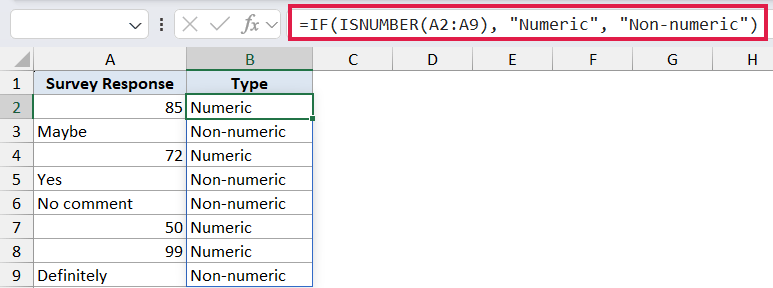
In the formula, ISNUMBER evaluates each value in the range and returns TRUE or FALSE. IF then picks the right label, “Numeric” for TRUE and “Non-numeric” for FALSE.
The numeric scores like 85, 72, 50, and 99 get the Numeric label. The text responses like Maybe, Yes, and Definitely get Non-numeric.
Example 4: Extract Only the Numbers with FILTER
Let’s step it up with a more useful scenario.
Sometimes you don’t just want to flag the numbers in a messy column, you want to pull them out into a clean second list. FILTER and ISNUMBER are made for this.
Below is the dataset. I have a column of imported values in column A. The export mixed labels, region names, and quarter tags into the same column as the actual numbers.
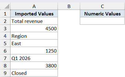
I want a clean list in column C that contains only the numeric entries, with the labels and text values left out.
Here is the formula:
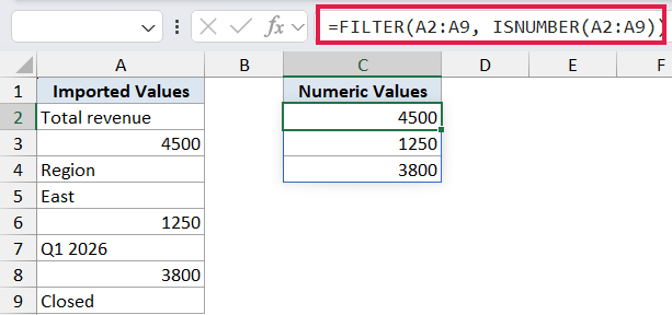
=FILTER(A2:A9, ISNUMBER(A2:A9))
How this formula works:
- ISNUMBER(A2:A9) builds a TRUE/FALSE array based on each value in the range.
- FILTER takes that array as its include test. It keeps only the rows where the test returns TRUE.
- The result spills into column C, showing just the numbers from the original list.
You get 4500, 1250, and 3800 in column C, which are the three numeric entries from the source column. Everything else gets dropped.
Example 5: Count Numeric Entries in a Column
Let’s wrap up with a quick count.
Sometimes you don’t need to label or extract anything, you just want to know how many cells in a range hold numbers. ISNUMBER inside SUM gives you that in one cell.
Below is the dataset. I have a column of survey submissions in column A. Some are numeric ratings, others are text answers.
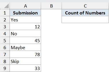
I want a single number in cell C2 that tells me how many entries in column A are numeric.
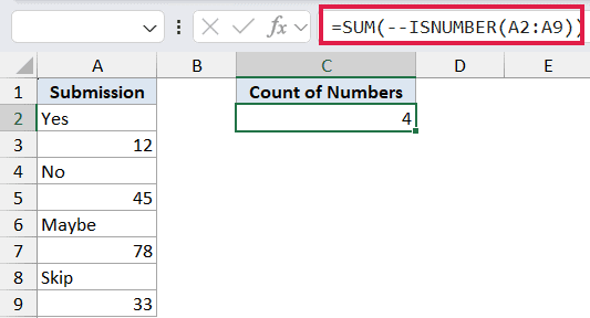
Here is the formula:
=SUM(--ISNUMBER(A2:A9))
How this formula works:
- ISNUMBER(A2:A9) returns an array of TRUE and FALSE values.
- The double minus (–) coerces those into 1s and 0s. TRUE becomes 1, FALSE becomes 0.
- SUM adds them up, giving you the count of numeric entries.
In this example, the result is 4, since the column has four numeric values (12, 45, 78, 33) and four text entries.
Pro Tip: If you just want a plain count of numbers, =COUNT(A2:A9) does the job in one step, since COUNT already ignores text and blanks. The ISNUMBER approach earns its keep when you want to combine the test with other conditions, or when you’re on a pre-365 version of Excel where SUM applied to an array needs Ctrl+Shift+Enter. In that case, swap SUM for SUMPRODUCT (=SUMPRODUCT(--ISNUMBER(A2:A9))) and it works without the array entry.
Tips & Common Mistakes
- Dates and times return TRUE. Dates in Excel are stored as serial numbers, so ISNUMBER treats them as numbers. If you want to flag dates specifically, you’ll need a different approach, like checking the cell format.
- Numbers stored as text return FALSE. If a number has a leading apostrophe (like
'1234) or was pasted in from another system as text, ISNUMBER will return FALSE. This is usually a signal that you need to convert the text to a real number using VALUE or a paste-special operation. - Blank cells return FALSE. ISNUMBER does not treat an empty cell as a number. If you want to check for empty cells specifically, use ISBLANK instead.
- Logical values return FALSE. TRUE and FALSE are not numbers as far as ISNUMBER is concerned. If you want to treat them as 1 and 0, wrap them in a math operation first.
- Pair it with SEARCH or FIND for substring checks. The
ISNUMBER(SEARCH(...))pattern is the most common idiom for “does this cell contain this text” in Excel. SEARCH is case-insensitive, FIND is case-sensitive. - Pair it with ISTEXT for the opposite check. ISTEXT is the complement of ISNUMBER for most cases. If you want to know whether something is text specifically, ISTEXT is the cleaner choice.
That covers the main ways ISNUMBER shows up in real spreadsheets. On its own it’s a one-line check, nothing fancy. But pair it with SEARCH for substring checks, IF for labels, FILTER to pull out only the numbers, or SUM to count them, and it quietly does a lot of work.
Related Excel Functions / Articles:
- COUNT Function in Excel
- ISBLANK Function in Excel
- How to Count Cells with Text in Excel?
- How to Extract Number from Text in Excel (Beginning, End, or Middle)
- Data Types in Excel
- How to Remove Numbers From Text in Excel
- Using IF Function with Dates in Excel (Easy Examples)
- How to Compare Two Cells in Excel? (Exact/Partial Match)
- ISNA Function in Excel