If you want a quick way to check whether a cell holds a text value or something else, the ISTEXT function is what you need.
It returns TRUE when the value is text and FALSE for anything else, including numbers, dates, errors, and blanks.
In Excel 365, you can also feed ISTEXT a range and the results spill into the cells below. In this article, I’ll show you how ISTEXT works with a few practical examples.
ISTEXT Syntax
Here is the syntax of the ISTEXT function:
=ISTEXT(value)
- value – The value you want to check. This can be a cell reference, a range, a literal in quotes, or a formula result. ISTEXT returns TRUE if the value is text, and FALSE for numbers, logical values, errors, or blank cells.
A small thing worth knowing. Numbers stored as text (often pasted in from other systems with a leading apostrophe) return TRUE, because Excel sees them as text strings. Dates return FALSE since dates are really numbers under the hood.
When to Use ISTEXT
Use this function when you need to:
- Flag cells that contain text in a mixed list of values
- Pull only the text entries out of a column using FILTER
- Build an IF formula that branches based on whether the input is text
- Count how many text values are in a range
- Drive conditional formatting that highlights text cells
Let me show you a few practical examples of how to use ISTEXT.
Example 1: Check a Mixed List for Text Values
Let’s start with a simple example to see ISTEXT in its most basic form.
Below is the dataset. I have a column of values in column A that came from a survey export. The list is mixed, with names, blank cells, dates, numbers, and a stray error.
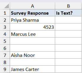
I want a TRUE or FALSE next to each value so I can see at a glance which entries are actual text.
Here is the formula:
=ISTEXT(A2:A9)
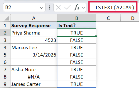
In the above formula, I’m feeding ISTEXT the entire range A2:A9 in one shot. Since ISTEXT spills in Excel 365, you only need to type the formula once in cell B2 and the results fill down to B9 automatically.
Names return TRUE, numbers and dates return FALSE, errors stay as errors, and blank cells return FALSE.
Pro Tip: If you are on an older version of Excel that does not support dynamic arrays, type =ISTEXT(A2) in B2 and drag it down through B9. Same result, just the legacy way of doing it.
Example 2: Extract Only the Text Entries with FILTER
Here’s another practical scenario where ISTEXT really earns its keep.
Below is the dataset. I have a column of customer feedback in column A. Some rows contain actual feedback comments, but the import dropped in some order numbers and timestamps too, so the list is messy.
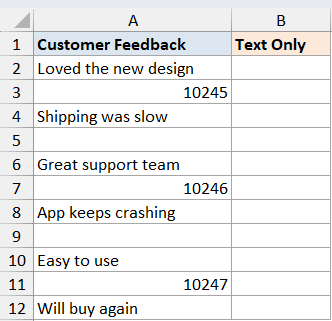
I want a clean second list in column C that contains only the text feedback, with the numbers and dates left out.
Here is the formula:
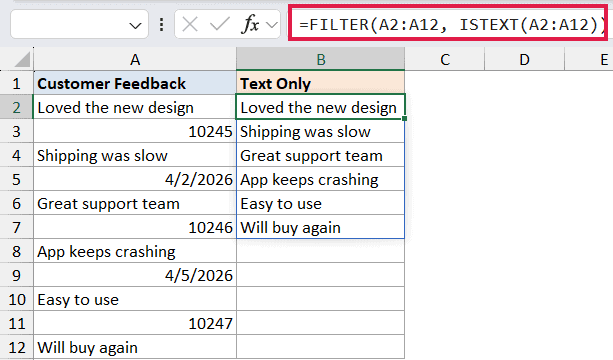
=FILTER(A2:A12, ISTEXT(A2:A12))
How this formula works:
- ISTEXT(A2:A12) returns an array of TRUE / FALSE values, one for each row.
- FILTER keeps only the rows where the array is TRUE, which means only the rows where the original value is text.
- The result spills down column C, with the order numbers and timestamps stripped out.
This is probably my favorite use of ISTEXT. A quick cleanup job that used to need a helper column collapses into one formula.
If you need to learn more about the FILTER side of this combo, check out the FILTER function tutorial.
A quick caveat. Numbers stored as text (with a leading apostrophe) will be picked up by ISTEXT as text, so they will show up in the filtered list too. If you want to exclude those as well, you would need an extra check.
Example 3: Label Each Row with IF and ISTEXT
Now let’s look at something more readable.
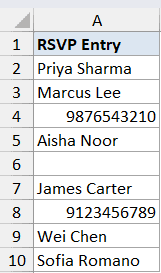
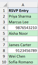
Below is the dataset. I have a column of event RSVPs in column A, where attendees were supposed to type their name but some typed a phone number or left the cell blank.
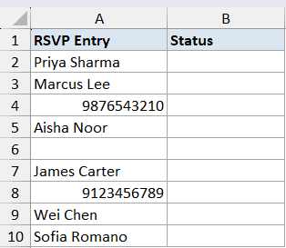
I want a friendly label next to each row that says “Name provided” when the entry is text and “Needs follow-up” when it is not.
Here is the formula:
=IF(ISTEXT(A2:A10), "Name provided", "Needs follow-up")
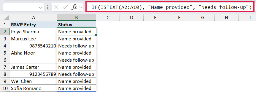
In the above formula, ISTEXT checks each cell in the range. When it returns TRUE, the IF function outputs “Name provided”. When it returns FALSE (because the entry is a number or the cell is blank), it outputs “Needs follow-up”.
The whole thing spills down column B in one go.
This pattern is also handy for data validation lists where you want a quick visual flag rather than a hard input restriction.
Example 4: Count Text Entries in a Column
Here’s a quick one. Sometimes you just want a count of how many cells in a range contain text.
Below is the dataset. I have a column of inventory SKUs in column A, where some entries are proper alphanumeric SKUs (like “AX-2204”) and some are just plain numbers from a legacy system.
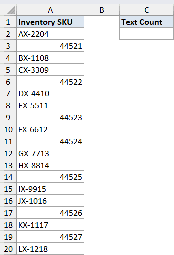
I want a single cell that tells me how many of the SKUs are stored as text.
Here is the formula:
=SUMPRODUCT(--ISTEXT(A2:A20))

How this formula works:
- ISTEXT(A2:A20) returns an array of TRUE and FALSE values.
- The double negative (
--) flips TRUE / FALSE into 1 / 0 so SUMPRODUCT can add them up. - SUMPRODUCT sums the 1s, which gives the count of text entries.
For more approaches to this kind of summary, see our full guide on count cells with text in Excel.
In Excel 365, you can also do this with =SUM(--ISTEXT(A2:A20)) since SUM now accepts arrays directly. Both work. The SUMPRODUCT version is the one that works in every version of Excel back to 2003, which is why you’ll see it everywhere.
Example 5: Highlight Text Cells with Conditional Formatting
Let’s wrap up with something visual.
I have the same mixed RSVP list from Example 3 in column A. Instead of writing a label in a second column, I want to highlight the cells that contain text directly.
I want the cells with names to turn green and leave everything else alone.
Here are the steps:
- Select the range A2:A10.
- Go to Home, then Conditional Formatting, then New Rule.
- Pick “Use a formula to determine which cells to format”.
- Enter the formula
=ISTEXT(A2). - Click Format, set the fill color to green, then click OK twice.
Here, the ISTEXT formula evaluates each cell in the selected range. Wherever it returns TRUE, conditional formatting paints the cell green. The numbers and blanks stay untouched.
Notice that the cell reference in the conditional formatting formula is A2 (the first cell of the selection), not the full range. Excel applies the formula to each cell in the range relative to its position, so you only point at the first cell.
Tips & Common Mistakes
- Numbers stored as text return TRUE. If a number has a leading apostrophe (like
'1234), ISTEXT will treat it as text. This is usually what you want, but it can surprise you when an imported column has numbers that look numeric but are actually stored as text. - Dates return FALSE. Dates in Excel are stored as serial numbers, so ISTEXT sees them as numbers, not text. If you want to flag text-formatted dates, you’ll need a different approach.
- Blank cells return FALSE. ISTEXT does not treat an empty cell as text. If you want to check for empty cells specifically, use ISBLANK instead.
- Formula results count. ISTEXT looks at the value in the cell, not the formula behind it. So
=ISTEXT(B2)where B2 holds=TEXT(100, "0.00")returns TRUE, because TEXT returns a text string. - Pair it with ISNUMBER for the opposite check. ISNUMBER is the complement of ISTEXT for most cases. If you want to know whether something is a number specifically, ISNUMBER is the cleaner choice.
- Know what counts as a text value in Excel. Anything that is not a number, formula, or logical value, including numbers that were imported as strings, is treated as text by ISTEXT.
That covers the main ways ISTEXT shows up in real spreadsheets. On its own it is just a TRUE / FALSE check, but pair it with FILTER, IF, or conditional formatting and it becomes a fast way to sort text from non-text in any messy column.
Worth keeping in your back pocket for the next time an import dumps a mixed bag into one column.
Related Excel Functions / Articles:
- COUNT Function in Excel
- SEARCH Function in Excel
- COUNTA Function in Excel
- How to Extract Number from Text in Excel (Beginning, End, or Middle)
- How to Remove Numbers From Text in Excel
- Data Types in Excel
- Using IF Function with Dates in Excel (Easy Examples)
- Multiple If Statements in Excel (Nested IFs, AND/OR) with Examples
- ISNA Function in Excel
- Check If a Cell Contains Text in Excel